This notebook is part of The Climate Laboratory by Brian E. J. Rose, University at Albany.
The amount of solar radiation incident on the top of the atmosphere (what we call the “insolation”) depends on
- latitude
- season
- time of day
This insolation is the primary driver of the climate system. Here we will examine the geometric factors that determine insolation, focussing primarily on the daily average values.
Solar zenith angle
We define the solar zenith angle as the angle between the local normal to Earth’s surface and a line between a point on Earth’s surface and the sun.

From the above figure (reproduced from Hartmann (1994)), the ratio of the shadow area to the surface area is equal to the cosine of the solar zenith angle.
Instantaneous solar flux
We can write the solar flux per unit surface area as
where is the mean distance for which the flux density (i.e. the solar constant) is measured, and is the actual distance from the sun.
Question:
- what factors determine ?
- under what circumstances would this ratio always equal 1?
Calculating the zenith angle
Just like the flux itself, the solar zenith angle depends latitude, season, and time of day.
Declination angle
The seasonal dependence can be expressed in terms of the declination angle of the sun: the latitude of the point on the surface of Earth directly under the sun at noon (denoted by ).
currenly varies between +23.45º at northern summer solstice (June 21) to -23.45º at northern winter solstice (Dec. 21).
Hour angle
The hour angle is defined as the longitude of the subsolar point relative to its position at noon.
Formula for zenith angle
With these definitions and some spherical geometry (see Appendix A of Hartmann’s book), we can express the solar zenith angle for any latitude , season, and time of day as
Sunrise and sunset
If then the sun is below the horizon and the insolation is zero (i.e. it’s night time!)
Sunrise and sunset occur when the solar zenith angle is 90º and thus . The above formula then gives
where is the hour angle at sunrise and sunset.
Polar night
Near the poles special conditions prevail. Latitudes poleward of 90º- are constantly illuminated in summer, when and are of the same sign. Right at the pole there is 6 months of perpetual daylight in which the sun moves around the compass at a constant angle above the horizon.
In the winter, and are of opposite sign, and latitudes poleward of 90º- are in perpetual darkness. At the poles, six months of daylight alternate with six months of daylight.
At the equator day and night are both 12 hours long throughout the year.
Daily average insolation
Substituting the expression for solar zenith angle into the insolation formula gives the instantaneous insolation as a function of latitude, season, and time of day:
which is valid only during daylight hours, , and otherwise (night).
To get the daily average insolation, we integrate this expression between sunrise and sunset and divide by 24 hours (or radians since we express the time of day in terms of hour angle):
which is easily integrated to get our formula for daily average insolation:
where the hour angle at sunrise/sunset must be in radians.
The daily average zenith angle
It turns out that, due to optical properties of the Earth’s surface (particularly bodies of water), the surface albedo depends on the solar zenith angle. It is therefore useful to consider the average solar zenith angle during daylight hours as a function of latidude and season.
The appropriate daily average here is weighted with respect to the insolation, rather than weighted by time. The formula is
Cronin (2014) also shows that the insolation-weighted value is a good choice for minimizing scattering bias under a variety of circumstances.
To calculate , we first note that the factor cancels out of the top and bottom of the above expression, leaving
With a bit of work, we can substitute in the expression for in terms of latitude , declination angle and hour angle and integrate the numerator and denominator of the above expression. I implement the resulting formulas in the Python code below
import numpy as np
import matplotlib.pyplot as plt
from numpy import sin,cos,tan,arccos,arcsin,arctan,pi,abs

lat = np.linspace(-90., 90, 500)
phi = np.deg2rad(lat)

declinations = {'21 December': -23.45,
                'Equinox': 0.,
                '21 June': 23.45}

def hour_angle_at_sunset(delta, phi):
    return np.where( abs(delta)-pi/2+abs(phi) < 0., # there is sunset/sunrise
              arccos(-tan(phi)*tan(delta)),
              # otherwise figure out if it's all night or all day
              np.where(phi*delta>0., pi, 0.) )

def insolation_weighted_coszen(delta, phi):
    h0 = hour_angle_at_sunset(delta, phi)
    denominator = h0*sin(phi)*sin(delta) + cos(phi)*cos(delta)*sin(h0)
    numerator = (h0*(2* sin(phi)**2*sin(delta)**2 + cos(phi)**2*cos(delta)**2) +
        cos(phi)*cos(delta)*sin(h0)*(4*sin(phi)*sin(delta) + cos(phi)*cos(delta)*cos(h0)))
    return numerator / denominator / 2

for label, delta in declinations.items():
    plt.plot(lat, np.rad2deg(arccos(insolation_weighted_coszen(np.deg2rad(delta), phi))), label=label)
plt.legend()
plt.grid()
plt.title('Insolation-weighted daily average solar zenith angle as a function of latitude');
plt.ylim(30,90);
plt.xlim(-90,90);
/var/folders/dl/j7hb106d36n501mrm8j646bxpf4y1c/T/ipykernel_1048/797907564.py:14: RuntimeWarning: invalid value encountered in arccos
arccos(-tan(phi)*tan(delta)),
/var/folders/dl/j7hb106d36n501mrm8j646bxpf4y1c/T/ipykernel_1048/797907564.py:23: RuntimeWarning: invalid value encountered in divide
return numerator / denominator / 2
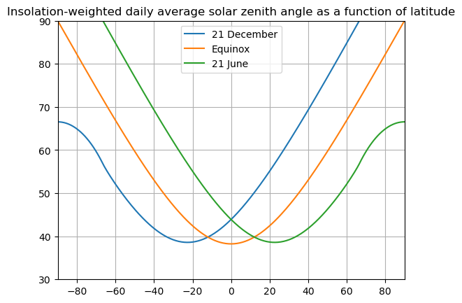
The figure above reproduces Figure 2.8 from Hartmann, 1994.
The average zenith angle is much higher at the poles than in the tropics. This contributes to the very high surface albedos observed at high latitudes.
Here are some examples calculating daily average insolation at different locations and times.
These all use a function called
daily_insolationin the package
climlab.solar.insolationto do the calculation. The code implements the above formulas to calculates daily average insolation anywhere on Earth at any time of year.
The code takes account of orbital parameters to calculate current Sun-Earth distance.
We can look up past orbital variations to compute their effects on insolation using the package
climlab.solar.orbitalSee the next lecture!
Using the daily_insolation function
from climlab import constants as const
from climlab.solar.insolation import daily_insolation
First, get a little help on using the daily_insolation function:
help(daily_insolation)Help on function daily_insolation in module climlab.solar.insolation:
daily_insolation(
lat,
day,
orb={'ecc': 0.017236, 'long_peri': 281.37, 'obliquity': 23.446},
S0=1365.2,
day_type=1,
days_per_year=365.2422
)
Compute daily average insolation given latitude, time of year and orbital parameters.
Orbital parameters can be interpolated to any time in the last 5 Myears with
``climlab.solar.orbital.OrbitalTable`` (see example above).
Longer orbital tables are available with ``climlab.solar.orbital.LongOrbitalTable``
Inputs can be scalar, ``numpy.ndarray``, or ``xarray.DataArray``.
The return value will be ``numpy.ndarray`` if **all** the inputs are ``numpy``.
Otherwise ``xarray.DataArray``.
**Function-call argument**
:param array lat: Latitude in degrees (-90 to 90).
:param array day: Indicator of time of year. See argument ``day_type``
for details about format.
:param dict orb: a dictionary with three members (as provided by
``climlab.solar.orbital.OrbitalTable``)
* ``'ecc'`` - eccentricity
* unit: dimensionless
* default value: ``0.017236``
* ``'long_peri'`` - longitude of perihelion (precession angle)
* unit: degrees
* default value: ``281.37``
* ``'obliquity'`` - obliquity angle
* unit: degrees
* default value: ``23.446``
:param float S0: solar constant
- unit: :math:`\textrm{W}/\textrm{m}^2`
- default value: ``1365.2``
:param int day_type: Convention for specifying time of year (+/- 1,2) [optional].
*day_type=1* (default):
day input is calendar day (1-365.24), where day 1
is January first. The calendar is referenced to the
vernal equinox which always occurs at day 80.
*day_type=2:*
day input is solar longitude (0-360 degrees). Solar
longitude is the angle of the Earth's orbit measured from spring
equinox (21 March). Note that calendar days and solar longitude are
not linearly related because, by Kepler's Second Law, Earth's
angular velocity varies according to its distance from the sun.
:raises: :exc:`ValueError`
if day_type is neither 1 nor 2
:returns: Daily average solar radiation in unit
:math:`\textrm{W}/\textrm{m}^2`.
Dimensions of output are ``(lat.size, day.size, ecc.size)``
:rtype: array
Code is fully vectorized to handle array input for all arguments.
Orbital arguments should all have the same sizes.
This is automatic if computed from
:func:`~climlab.solar.orbital.OrbitalTable.lookup_parameters`
For more information about computation of solar insolation see the
:ref:`Tutorial` chapter.
.. note::
Calling ``insolation = daily_insolation(lat, day, orb, S0)`` is equivalent to::
coszen, irradiance_factor = daily_insolation_factors(lat, day, orb)
insolation = S0 * irradiance_factor * coszen
Computing the zenith angle with ``daily_insolation_factors`` allows for
optional time averaging choices which may be important for certain
radiative transfer calculations that are sensitive to zenith angle.
Here are a few simple examples.
First, compute the daily average insolation at 45ºN on January 1:
daily_insolation(45,1)np.float64(123.95321551807461)Same location, July 1:
daily_insolation(45,181)np.float64(482.356497522712)We could give an array of values. Let’s calculate and plot insolation at all latitudes on the spring equinox = March 21 = Day 80
lat = np.linspace(-90., 90., 30)
Q = daily_insolation(lat, 80)
fig, ax = plt.subplots()
ax.plot(lat,Q)
ax.set_xlim(-90,90); ax.set_xticks([-90,-60,-30,-0,30,60,90])
ax.set_xlabel('Latitude')
ax.set_ylabel('W/m2')
ax.grid()
ax.set_title('Daily average insolation on March 21')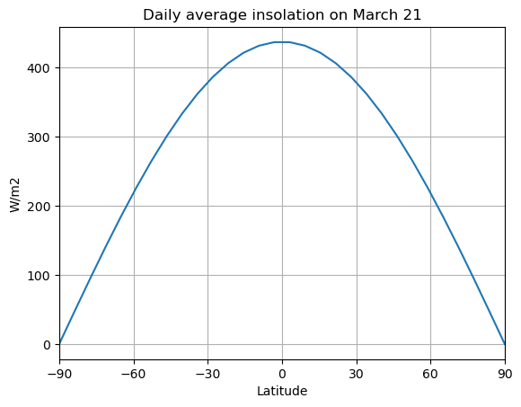
In-class exercises
Try to answer the following questions before reading the rest of these notes.
- What is the daily insolation today here at Albany (latitude 42.65ºN)?
- What is the annual mean insolation at the latitude of Albany?
- At what latitude and at what time of year does the maximum daily insolation occur?
- What latitude is experiencing either polar sunrise or polar sunset today?
Calculate an array of insolation over the year and all latitudes (for present-day orbital parameters). We’ll use a dense grid in order to make a nice contour plot
lat = np.linspace( -90., 90., 500)
numpoints = 365.
days = np.linspace(1., numpoints, 365)/numpoints * const.days_per_year

Q = daily_insolation( lat, days )
And make a contour plot of Q as function of latitude and time of year.
fig, ax = plt.subplots(figsize=(10,8))
CS = ax.contour( days, lat, Q , levels = np.arange(0., 600., 50.) )
ax.clabel(CS, CS.levels, inline=True, fmt='%1.0f', fontsize=10)
ax.set_xlabel('Days since January 1', fontsize=16 )
ax.set_ylabel('Latitude', fontsize=16 )
ax.set_title('Daily average insolation', fontsize=24 )
ax.contourf ( days, lat, Q, levels=[-1000., 0.], colors='k' )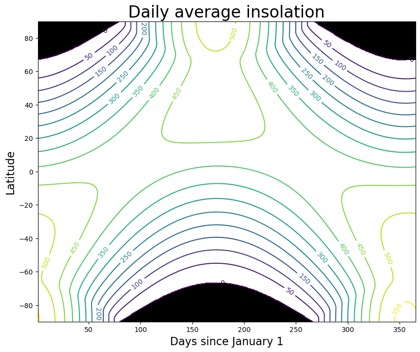
Time and space averages
Take the area-weighted global, annual average of Q...
Qaverage = np.average(np.mean(Q, axis=1), weights=np.cos(np.deg2rad(lat)))
print( 'The annual, global average insolation is %.2f W/m2.' %Qaverage)
The annual, global average insolation is 341.35 W/m2.
Also plot the zonally averaged insolation at a few different times of the year:
summer_solstice = 170
winter_solstice = 353
fig, ax = plt.subplots(figsize=(10,8))
ax.plot( lat, Q[:,(summer_solstice, winter_solstice)] );
ax.plot( lat, np.mean(Q, axis=1), linewidth=2 )
ax.set_xbound(-90, 90)
ax.set_xticks( range(-90,100,30) )
ax.set_xlabel('Latitude', fontsize=16 );
ax.set_ylabel('Insolation (W m$^{-2}$)', fontsize=16 );
ax.grid()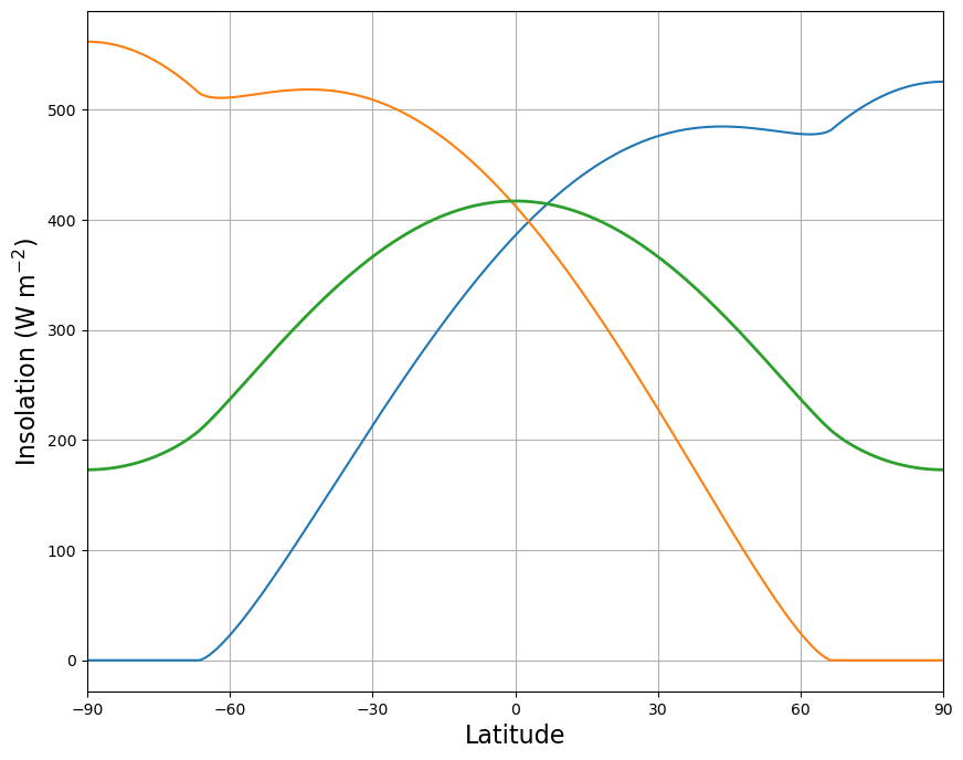
Credits
This notebook is part of The Climate Laboratory, an open-source textbook developed and maintained by Brian E. J. Rose, University at Albany.
It is licensed for free and open consumption under the Creative Commons Attribution 4.0 International (CC BY 4.0) license.
Development of these notes and the climlab software is partially supported by the National Science Foundation under award AGS-1455071 to Brian Rose. Any opinions, findings, conclusions or recommendations expressed here are mine and do not necessarily reflect the views of the National Science Foundation.
- Hartmann, D. L. (1994). Global Physical Climatology (Vol. 56). Academic Press.
- Cronin, T. W. (2014). On the Choice of Average Solar Zenith Angle. J. Atmos. Sci., 71, 2994–3003. 10.1175/JAS-D-13-0392.1