This notebook is part of The Climate Laboratory by Brian E. J. Rose, University at Albany.
Subsections marked with the asterisk * are more detailed mathematical discussions which can be skipped by the first-time reader.
In the previous lectures we have seen how heat transport by winds and ocean currents acts to COOL the tropics and WARM the poles. The observed temperature gradient is a product of both the insolation and the heat transport!
We were able to ignore this issue in our models of the global mean temperature, because the transport just moves energy around between latitude bands – does not create or destroy energy.
But if want to move beyond the global mean and create models of the equator-to-pole temperature structure, we cannot ignore heat transport. Has to be included somehow!
This leads to us the old theme of simulation versus parameterization.
Complex climate models like the CESM simulate the heat transport by solving the full equations of motion for the atmosphere (and ocean too, if coupled).
Simulation of synoptic-scale variability in CESM
Let’s revisit an animation of the global 6-hourly sea-level pressure field from our slab ocean simulation with CESM. (We first saw this back in the notes on Climate Systems and Climate Models)
from IPython.display import YouTubeVideo
YouTubeVideo('As85L34fKYQ')All these traveling weather systems tend to move warm, moist air poleward and cold, dry air equatorward. There is thus a net poleward energy transport.
A model like this needs to simulate the weather in order to model the heat transport.
A simpler statistical approach
Let’s emphasize: the most important role for heat transport by winds and ocean currents is to more energy from where it’s WARM to where it’s COLD, thereby reducing the temperature gradient (equator to pole) from what it would be if the planet were in radiative-convective equilibrium everywhere with no north-south motion.
This is the basis for the parameterization of heat transport often used in simple climate models.
Discuss analogy with molecular heat conduction: metal rod with one end in the fire.
Define carefully temperature gradient dTs / dy Measures how quickly the temperature decreases as we move northward (negative in NH, positive in SH)
In any conduction or diffusion process, the flux (transport) of a quantity is always DOWN-gradient (from WARM to COLD).
So our parameterization will look like
Where is some positive number “diffusivity of the climate system”.
Definition
Last time we wrote down an energy budget for a thin zonal band centered at latitude :
where we have written every term as an explicit function of latitude to remind ourselves that this is a local budget, unlike the zero-dimensional global budget we considered at the start of the course.
Let’s now formally introduce a parameterization that approximates the heat transport as a down-gradient diffusion process:
With a parameter for the diffusivity or thermal conductivity of the climate system, a number in W m ºC.
The value of will be chosen to match observations – i.e. tuned.
Notice that we have explicitly chosen to the use surface temperature gradient to set the heat transport. This is a convenient (and traditional) choice to make, but it is not the only possibility! We could instead tune our parameterization to some measure of the free-tropospheric temperature gradient.
The diffusive parameterization in the planetary energy budget
Plug the parameterization into our energy budget to get
If we assume that is a constant (does not vary with latitude), then this simplifies to
Surface temperature is a good measure of column heat content
Let’s now make the same assumption we made [back at the beginning of the course](Lecture01 -- Planetary energy budget.ipynb) when we first wrote down the zero-dimensional EBM.
Most of the heat capacity is in the oceans, so that the energy content of each column is proportional to surface temperature:
where is effective heat capacity of the atmosphere - ocean column, in units of J m K. Here we are writing are a function of latitude so that our model is general enough to allow different land-ocean fractions at different latitudes.
A heat equation for surface temperature
Now our budget becomes a PDE for the surface temperature :
Notice that if we were NOT on a spherical planet and didn’t have to worry about the changing size of latitude circles, this would look something like
with in m s.
Does equation look familiar?
This is the heat equation, one of the central equations in classical mathematical physics.
This equation describes the behavior of a diffusive system, i.e. how mixing by random molecular motion smears out the temperature.
In our case, the analogy is between the random molecular motion of a metal rod, and the net mixing / stirring effect of weather systems.
* Take the global average...
Take the integral of each term.
The global average of the last term (heat transport) must go to zero (why?)
Therefore this reduces to our familiar zero-dimensional EBM.
climlab has a pre-defined process for solving the meridional diffusion equation. Let’s look at a simple example in which diffusion is the ONLY process that changes the temperature.
The equation we’re going to solve here is
(i.e. the EBM equation without any radiation terms)
%matplotlib inline
import numpy as np
import matplotlib.pyplot as plt
import climlab
from climlab import constants as const
# First define an initial temperature field
# that is warm at the equator and cold at the poles
# and varies smoothly with latitude in between
from climlab.utils import legendre
sfc = climlab.domain.zonal_mean_surface(num_lat=90, water_depth=10.)
lat = sfc.lat.points
initial = 12. - 40. * legendre.P2(np.sin(np.deg2rad(lat)))
fig, ax = plt.subplots()
ax.plot(lat, initial)
ax.set_xlabel('Latitude')
ax.set_ylabel('Temperature (deg C)');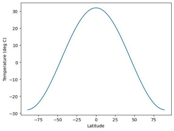
##  Set up the climlab diffusion process

# make a copy of initial so that it remains unmodified
Ts = climlab.Field(np.array(initial), domain=sfc)
# thermal diffusivity in W/m**2/degC
D = 0.55
# create the climlab diffusion process
#  setting the diffusivity and a timestep of ONE MONTH
d = climlab.dynamics.MeridionalHeatDiffusion(name='Diffusion',
            state=Ts, D=D, timestep=const.seconds_per_month)
print(d)
climlab Process of type <class 'climlab.dynamics.meridional_heat_diffusion.MeridionalHeatDiffusion'>.
State variables and domain shapes:
default: (90, 1)
The subprocess tree:
Diffusion: <class 'climlab.dynamics.meridional_heat_diffusion.MeridionalHeatDiffusion'>
#  We are going to step forward one month at a time
#  and store the temperature each time
n_iter = 5
temp = np.zeros((Ts.size, n_iter+1))
temp[:, 0] = np.squeeze(Ts)
for n in range(n_iter):
    d.step_forward()
    temp[:, n+1] = np.squeeze(Ts)
# Now plot the temperatures
fig,ax = plt.subplots()
ax.plot(lat, temp)
ax.set_xlabel('Latitude')
ax.set_ylabel('Temperature (deg C)')
ax.legend(range(n_iter+1)); ax.grid();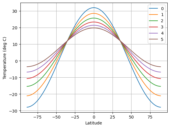
At each timestep, the warm temperatures get cooler (at the equator) while the cold polar temperatures get warmer!
Diffusion is acting to reduce the temperature gradient.
If we let this run a long time, what should happen??
Try it yourself and find out!
* Mathematical aside: the Legendre Polynomials
Here we have used a function called the “2nd Legendre polynomial”, defined as
where we have also set
Just turns out to be a useful mathematical description of the relatively smooth changes in things like annual-mean insolation from equator to pole.
In fact these are so useful that they are coded up in a special module within climlab:
x = np.linspace(-1,1)
fig,ax = plt.subplots()
ax.plot(x, legendre.P2(x))
ax.set_title('$P_2(x)$')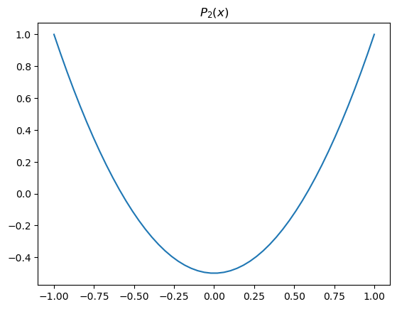
To turn our budget into a model, we need specific parameterizations that link the radiation ASR and OLR to surface temperature (the state variable for our model).
In mathematical terms, we want to express this as a closed equation for surface temperature .
For now, we will assume that the planetary albedo is fixed (does not depend on temperature). Therefore the entire shortwave term is a fixed source term in our budget. It varies in space and time but does not depend on .
Note that the solar term is (at least in annual average) larger at equator than poles… and transport term acts to flatten out the temperatures.
Parameterizing the longwave radiation
Now, we almost have a model we can solve for T! Just need to express the OLR in terms of temperature.
So… what’s the link between OLR and temperature????
[ discuss ]
We spent a good chunk of the course looking at this question, and developed a model of a vertical column of air.
We are trying now to build a model of the equator-to-pole (or pole-to-pole) temperature structure.
We COULD use an array of column models, representing temperature as a function of height and latitude (and time).
But instead, we will keep things simple, one spatial dimension at a time.
Introduce the following simple parameterization:
With:
the zonal average surface temperature in ºC
is a constant in W m
is a constant in W m ºC
Think of as an inverse measure of the greenhouse gas amount (Why?).
The parameter is closely related to the climate feedback parameter that we defined a while back. The only difference is that in the EBM we are going to explicitly separate the albedo feedback from all other radiative feedbacks.
OLR versus surface temperature in NCEP Reanalysis data
Let’s look at the data to find reasonable values for and .
import xarray as xr
## The NOAA ESRL server is shutdown! January 2019
ncep_url = "http://www.esrl.noaa.gov/psd/thredds/dodsC/Datasets/ncep.reanalysis.derived/"
ncep_Ts = xr.open_dataset( ncep_url + "surface_gauss/skt.sfc.mon.1981-2010.ltm.nc", decode_times=False)
#url = 'http://apdrc.soest.hawaii.edu:80/dods/public_data/Reanalysis_Data/NCEP/NCEP/clima/'
#ncep_Ts = xr.open_dataset(url + 'surface_gauss/skt')
lat_ncep = ncep_Ts.lat; lon_ncep = ncep_Ts.lon
print( ncep_Ts)
<xarray.Dataset> Size: 2MB
Dimensions: (lon: 192, time: 12, lat: 94, nbnds: 2)
Coordinates:
* lon (lon) float32 768B 0.0 1.875 3.75 ... 354.4 356.2 358.1
* time (time) float64 96B -6.571e+05 -6.57e+05 ... -6.567e+05
* lat (lat) float32 376B 88.54 86.65 84.75 ... -86.65 -88.54
Dimensions without coordinates: nbnds
Data variables:
climatology_bounds (time, nbnds) float64 192B ...
skt (time, lat, lon) float32 866kB ...
valid_yr_count (time, lat, lon) float32 866kB ...
Attributes:
title: 4x daily NMC reanalysis
description: Data is from NMC initialized reanalysis\n...
platform: Model
Conventions: COARDS
not_missing_threshold_percent: minimum 3% values input to have non-missi...
history: Created 2011/07/12 by doMonthLTM\nConvert...
dataset_title: NCEP-NCAR Reanalysis 1
References: http://www.psl.noaa.gov/data/gridded/data...
_NCProperties: version=2,netcdf=4.6.3,hdf5=1.10.5
#  Take the annual and zonal average!
Ts_ncep_annual = ncep_Ts.skt.mean(dim=('lon','time'))
# TOA radiation data
ncep_ulwrf = xr.open_dataset( ncep_url + "other_gauss/ulwrf.ntat.mon.1981-2010.ltm.nc", decode_times=False)
ncep_dswrf = xr.open_dataset( ncep_url + "other_gauss/dswrf.ntat.mon.1981-2010.ltm.nc", decode_times=False)
ncep_uswrf = xr.open_dataset( ncep_url + "other_gauss/uswrf.ntat.mon.1981-2010.ltm.nc", decode_times=False)
#ncep_ulwrf = xr.open_dataset(url + "other_gauss/ulwrf")
#ncep_dswrf = xr.open_dataset(url + "other_gauss/dswrf")
#ncep_uswrf = xr.open_dataset(url + "other_gauss/uswrf")
OLR_ncep_annual = ncep_ulwrf.ulwrf.mean(dim=('lon','time'))
ASR_ncep_annual = (ncep_dswrf.dswrf - ncep_uswrf.uswrf).mean(dim=('lon','time'))# Use a linear regression package to compute best fit for the slope and intercept
from scipy.stats import linregress
slope, intercept, r_value, p_value, std_err = linregress(Ts_ncep_annual, OLR_ncep_annual)
print( 'Best fit is A = %0.0f W/m2 and B = %0.1f W/m2/degC' %(intercept, slope))Best fit is A = 214 W/m2 and B = 1.6 W/m2/degC
We’re going to plot the data and the best fit line, but also another line using these values:
#  More standard values
A = 210.
B = 2.
fig, ax1 = plt.subplots(figsize=(8,6))
ax1.plot( Ts_ncep_annual, OLR_ncep_annual, 'o' , label='data')
ax1.plot( Ts_ncep_annual, intercept + slope * Ts_ncep_annual, 'k--', label='best fit')
ax1.plot( Ts_ncep_annual, A + B * Ts_ncep_annual, 'r--', label='B=2')
ax1.set_xlabel('Surface temperature (C)', fontsize=16)
ax1.set_ylabel('OLR (W m$^{-2}$)', fontsize=16)
ax1.set_title('OLR versus surface temperature from NCEP reanalysis', fontsize=18)
ax1.legend(loc='upper left')
ax1.grid()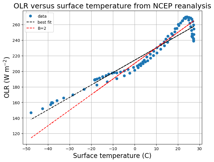
Discuss these curves...
Suggestion of at least 3 different regimes with different slopes (cold, medium, warm).
Unbiased “best fit” is actually a poor fit over all the intermediate temperatures.
The astute reader will note that... by taking the zonal average of the data before the regression, we are biasing this estimate toward cold temperatures. [WHY?]
Let’s take these reference values:
Checking the global average
Note that in the global average, recall
And so this parameterization gives
And the observed global mean is So this is consistent.
Relationship between and feedback parameters
Recall that when we looked at climate forcing and feedback, we said that overall response to a forcing in W m is
and where is the overall climate feedback parameter:
and
W m K is the no-feedback climate response
is the sum of all radiative feedbacks, defined to be positive for amplifying processes.
More positive feedbacks thus mean that is a smaller number, which means the response to a given forcing is larger!
Here in the EBM the parameter plays the same role as -- a smaller number means a more sensitive model.
Our estimate thus implies that the sum of all LW feedback processes (including water vapor, lapse rates and clouds) is
Looking back at the chart of feedback parameter values from GCMs, does this seem plausible?
Putting the equation together
Putting the above OLR parameterization into our budget equation gives
This is the equation for a very important and useful simple model of the climate system. It is typically referred to as the (one-dimensional) Energy Balance Model.
(although as we have seen over and over, EVERY climate model is actually an “energy balance model” of some kind)
Also for historical reasons this is often called the Budyko-Sellers model, after Budyko and Sellers who both (independently of each other) published influential papers on this subject in 1969 Budyko, 1969Sellers, 1969.
Recap: parameters in this model are
C: heat capacity in J m ºC
A: longwave emission at 0ºC in W m
B: increase in emission per degree, in W m ºC
D: horizontal (north-south) diffusivity of the climate system in W m ºC
We also need to specify the albedo.
Observed albedo
Let’s go back to the NCEP Reanalysis data to see how planetary albedo actually varies as a function of latitude.
days = np.linspace(1.,50.)/50 * const.days_per_year
Qann_ncep = climlab.solar.insolation.daily_insolation(lat_ncep, days ).mean(dim='day')
albedo_ncep = 1 - ASR_ncep_annual / Qann_ncep

albedo_ncep_global = np.average(albedo_ncep, weights=np.cos(np.deg2rad(lat_ncep)))
print( 'The annual, global mean planetary albedo is %0.3f' %albedo_ncep_global)
fig,ax = plt.subplots()
ax.plot(lat_ncep, albedo_ncep)
ax.grid();
ax.set_xlabel('Latitude')
ax.set_ylabel('Albedo');The annual, global mean planetary albedo is 0.354
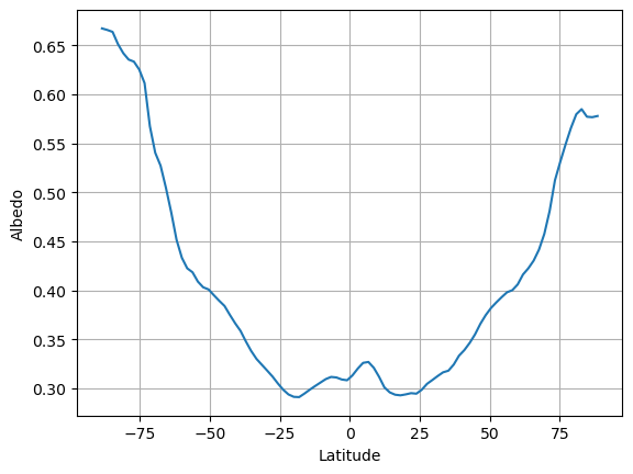
The albedo increases markedly toward the poles.
There are several reasons for this:
Surface snow and ice increase toward the poles
Cloudiness is an important (but complicated) factor.
Albedo increases with solar zenith angle (the angle at which the direct solar beam strikes a surface)
Approximating the observed albedo with a smooth function
Like temperature and insolation, this can be approximated by a smooth function that increases with latitude:
where is the 2nd Legendre polynomial (see above).
In effect we are using a truncated series expansion of the full meridional structure of . is the global average, and is proportional to the equator-to-pole gradient in .
We will set
# Add a new curve to the previous figure
a0 = albedo_ncep_global
a2 = 0.25
ax.plot(lat_ncep, a0 + a2 * legendre.P2(np.sin(np.deg2rad(lat_ncep))))
fig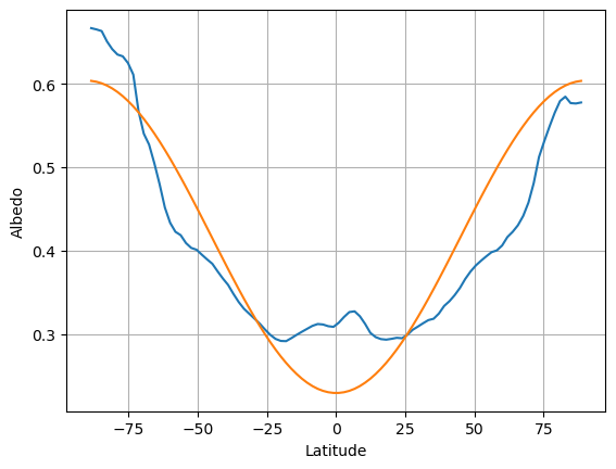
Of course we are not fitting all the details of the observed albedo curve. But we do get the correct global mean a reasonable representation of the equator-to-pole gradient in albedo.
For now, we will be focusing on the annual mean model.
For the insolation, we set , the annual mean value (large at equator, small at pole).
* Mathematical details: deriving the annual mean model
Suppose we take the annual mean of the planetary energy budget.
If the albedo is fixed, then the average is pretty simple. Our EBM equation is purely linear, so the change over one year is just
where is the annual mean surface temperature, and is the annual mean insolation (both functions of latitude).
Notice that once we average over the seasonal cycle, there are no time-dependent forcing terms. The temperature will just evolve toward a steady equilibrium.
The equilibrium temperature is then the solution of this Ordinary Differential Equation (setting above):
You will often see this equation written in terms of the independent variable
which is 0 at the equator and at the poles. Substituting this for , noting that and rearranging a bit gives
This is actually a 2nd order ODE, and actually a 2-point Boundary Value Problem for the temperature , where the boundary conditions are no-flux at the boundaries (usually the poles).
This form can be convenient for analytical solutions. As we will see, the non-dimensional number is a very important measure of the efficiency of heat transport in the climate system. We will return to this later.
Numerical solutions of the time-dependent EBM
We will leave the time derivative in our model, because this is the most convenient way to find the equilibrium solution!
There is code available in climlab to solve the diffusive EBM.
Animating the adjustment of annual mean EBM to equilibrium
Before looking at the details of how to set up an EBM in climlab, let’s look at an animation of the adjustment of the model (its temperature and energy budget) from an isothermal initial condition.
For reference, all the code necessary to generate the animation is here in the notebook.
#  Some imports needed to make and display animations
from IPython.display import HTML
from matplotlib import animation

def setup_figure():
    templimits = -20,32
    radlimits = -340, 340
    htlimits = -6,6
    latlimits = -90,90
    lat_ticks = np.arange(-90,90,30)

    fig, axes = plt.subplots(3,1,figsize=(8,10))
    axes[0].set_ylabel('Temperature (deg C)')
    axes[0].set_ylim(templimits)
    axes[1].set_ylabel('Energy budget (W m$^{-2}$)')
    axes[1].set_ylim(radlimits)
    axes[2].set_ylabel('Heat transport (PW)')
    axes[2].set_ylim(htlimits)
    axes[2].set_xlabel('Latitude')
    for ax in axes: ax.set_xlim(latlimits); ax.set_xticks(lat_ticks); ax.grid()
    fig.suptitle('Diffusive energy balance model with annual-mean insolation', fontsize=14)
    return fig, axes

def initial_figure(model):
    #  Make figure and axes
    fig, axes = setup_figure()
    # plot initial data
    lines = []
    lines.append(axes[0].plot(model.lat, model.Ts)[0])
    lines.append(axes[1].plot(model.lat, model.ASR, 'k--', label='SW')[0])
    lines.append(axes[1].plot(model.lat, -model.OLR, 'r--', label='LW')[0])
    lines.append(axes[1].plot(model.lat, model.net_radiation, 'c-', label='net rad')[0])
    lines.append(axes[1].plot(model.lat, model.heat_transport_convergence, 'g--', label='dyn')[0])
    lines.append(axes[1].plot(model.lat,
            model.net_radiation+model.heat_transport_convergence, 'b-', label='total')[0])
    axes[1].legend(loc='upper right')
    lines.append(axes[2].plot(model.lat_bounds, model.heat_transport)[0])
    lines.append(axes[0].text(60, 25, 'Day 0'))
    return fig, axes, lines

def animate(day, model, lines):
    model.step_forward()
    #  The rest of this is just updating the plot
    lines[0].set_ydata(model.Ts)
    lines[1].set_ydata(model.ASR)
    lines[2].set_ydata(-model.OLR)
    lines[3].set_ydata(model.net_radiation)
    lines[4].set_ydata(model.heat_transport_convergence)
    lines[5].set_ydata(model.net_radiation+model.heat_transport_convergence)
    lines[6].set_ydata(model.heat_transport)
    lines[-1].set_text('Day {}'.format(int(model.time['days_elapsed'])))
    return lines
# A model starting from isothermal initial conditions
e = climlab.EBM_annual()
e.Ts[:] = 15. # in degrees Celsius
e.compute_diagnostics()# Plot initial data
fig, axes, lines = initial_figure(e)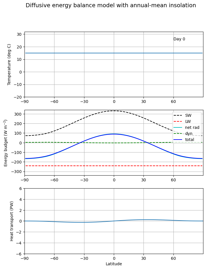
ani = animation.FuncAnimation(fig, animate, frames=np.arange(1, 100), fargs=(e, lines))HTML(ani.to_html5_video())This animation lets us visualize the competition between the radiation which is trying to warm the tropics and cool the poles, and the dynamics which is doing the opposite.
This is very much analogous to the competition between radiation and convection we saw in our study of radiative-convective equilibrium in a single vertical column.
Example EBM using climlab
Here is a simple example using the parameter values we just discussed.
For simplicity, this model will use the annual mean insolation, so the forcing is steady in time.
We haven’t yet selected an appropriate value for the diffusivity . Let’s just try something and see what happens:
D = 0.1
model = climlab.EBM_annual(name='EBM', A=210, B=2, D=D, a0=0.354, a2=0.25)
print(model)
climlab Process of type <class 'climlab.model.ebm.EBM_annual'>.
State variables and domain shapes:
Ts: (90, 1)
The subprocess tree:
EBM: <class 'climlab.model.ebm.EBM_annual'>
LW: <class 'climlab.radiation.aplusbt.AplusBT'>
insolation: <class 'climlab.radiation.insolation.AnnualMeanInsolation'>
albedo: <class 'climlab.surface.albedo.P2Albedo'>
SW: <class 'climlab.radiation.absorbed_shorwave.SimpleAbsorbedShortwave'>
diffusion: <class 'climlab.dynamics.meridional_heat_diffusion.MeridionalHeatDiffusion'>
# The model object stores a dictionary of important parameters
model.param
{'timestep': 350632.51200000005,
'S0': 1365.2,
's2': -0.48,
'A': 210,
'B': 2,
'D': 0.1,
'water_depth': 10.0,
'a0': 0.354,
'a2': 0.25}# Run it out long enough to reach equilibrium
model.integrate_years(10)Integrating for 900 steps, 3652.4220000000005 days, or 10 years.
Total elapsed time is 9.999999999999863 years.
Comparison of the equilibrium climate to observations
fig, axes = plt.subplots(1,2, figsize=(12,4))
ax = axes[0]
ax.plot(model.lat, model.Ts, label=('D = %0.1f' %D))
ax.plot(lat_ncep, Ts_ncep_annual, label='obs')
ax.set_ylabel('Temperature (degC)')
ax = axes[1]
energy_in = np.squeeze(model.ASR - model.OLR)
ax.plot(model.lat, energy_in, label=('D = %0.1f' %D))
ax.plot(lat_ncep, ASR_ncep_annual - OLR_ncep_annual, label='obs')
ax.set_ylabel('Net downwelling radiation at TOA (W m$^{-2}$)')
for ax in axes:
    ax.set_xlabel('Latitude'); ax.legend(); ax.grid();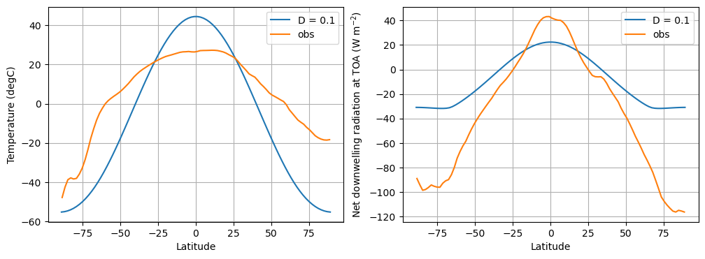
def inferred_heat_transport( energy_in, lat_deg ):
    '''Returns the inferred heat transport (in PW) by integrating the net energy imbalance from pole to pole.'''
    from scipy import integrate
    from climlab import constants as const
    lat_rad = np.deg2rad( lat_deg )
    return ( 1E-15 * 2 * np.pi * const.a**2 *
            integrate.cumulative_trapezoid( np.cos(lat_rad)*energy_in,
            x=lat_rad, initial=0. ) )
fig, ax = plt.subplots()
ax.plot(model.lat, inferred_heat_transport(energy_in, model.lat), label=('D = %0.1f' %D))
ax.set_ylabel('Heat transport (PW)')
ax.legend(); ax.grid()
ax.set_xlabel('Latitude')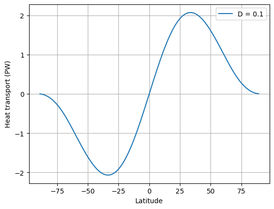
The upshot: compared to observations, this model has a much too large equator-to-pole temperature gradient, and not enough poleward heat transport!
Apparently we need to increase the diffusivity to get a better fit.
What is the optimal value for ?
We want to choose a value of that gives a reasonable approximation to observations:
ºC between equator and pole
PW (peak heat transport)
I can do some trial and error. For no particular reason, let’s start with W m ºC, and see how close we get to these targets.
ebm = climlab.EBM_annual(num_lat=40, A=210, B=2, a0=0.354, a2=0.25, D=1.)
ebm.integrate_years(20.)
Integrating for 1800 steps, 7304.844000000001 days, or 20.0 years.
Total elapsed time is 19.99999999999943 years.
Note that we have an array of 40 surface temperature values on our latitude grid:
# I can always look at the model variables as xarray objects if it's helpful
climlab.to_xarray(ebm.Ts)I can calculate the equator-to-pole temperature difference just by looking for the largest and smallest values:
deltaT = np.max(ebm.Ts) - np.min(ebm.Ts)
print(deltaT)
32.84075522594026
And the heat transport is a diagnostic calculated by the model:
# the poleward heat transport in PW
ebm.heat_transport
Field([[ 0.00000000e+00],
[-9.18904284e-02],
[-3.64621108e-01],
[-8.09080950e-01],
[-1.40900546e+00],
[-2.13887046e+00],
[-2.95710444e+00],
[-3.80557880e+00],
[-4.62917406e+00],
[-5.37363147e+00],
[-5.98702816e+00],
[-6.42232424e+00],
[-6.64021012e+00],
[-6.61185866e+00],
[-6.32125688e+00],
[-5.76684312e+00],
[-4.96224035e+00],
[-3.93595867e+00],
[-2.73003339e+00],
[-1.39766258e+00],
[-1.04149850e-08],
[ 1.39766256e+00],
[ 2.73003337e+00],
[ 3.93595865e+00],
[ 4.96224033e+00],
[ 5.76684310e+00],
[ 6.32125687e+00],
[ 6.61185864e+00],
[ 6.64021011e+00],
[ 6.42232423e+00],
[ 5.98702816e+00],
[ 5.37363146e+00],
[ 4.62917406e+00],
[ 3.80557879e+00],
[ 2.95710444e+00],
[ 2.13887046e+00],
[ 1.40900546e+00],
[ 8.09080950e-01],
[ 3.64621108e-01],
[ 9.18904284e-02],
[ 0.00000000e+00]])I am mostly interested in finding its peak value:
np.max(ebm.heat_transport)Field(6.64021011)So... for a diffusivity parameter W m ºC I get the following results:
C
PW
Comparing to our observational targets, this is too much heat transport and too small temperature gradient!
Class exercise: crowd-sourcing the optical value for 
Repeat these calculations with some different values of . We’ll crowd-source the optimal value that best matches our observational targets.
Tabulate our crowd-sourced results!
The pandas package is very very useful for working with spreadsheet-style data in Python.
import pandas as pd

classdata = pd.DataFrame([
              [1., 32.8, 6.64],
              # add more datasets in the same order: D, T, H
              #[, ,],
             ],
            columns=[r'$D$', r'$\Delta T$', r'$\mathcal{H}_{max}$'])
classdataNow we can do fun things like make a scatterplot of the data. The pd.DataFrame object lets us make use of the labels in our dataset to make the code simpler and easier to read:
fig, axes = plt.subplots(2,1)
classdata.plot.scatter(x=r'$D$', y=r'$\Delta T$', ax=axes[0])
classdata.plot.scatter(x=r'$D$', y=r'$\mathcal{H}_{max}$', ax=axes[1])
<Axes: xlabel='$D$', ylabel='$\\mathcal{H}_{max}$'>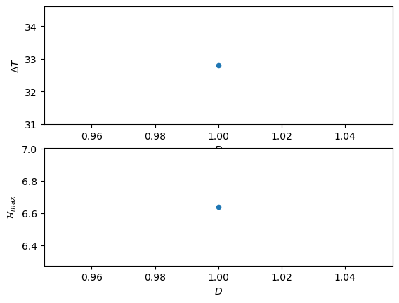
Is it starting to become clear what value we should choose?
A more systematic search
Do this as in-class investigation for a more advanced exercise
Solve the annual-mean EBM (integrate out to equilibrium) over a range of different diffusivity parameters.
Make three plots:
Global-mean temperature as a function of
Equator-to-pole temperature difference as a function of
Maximum poleward heat transport as a function of
Choose a value of that gives a reasonable approximation to observations:
ºC
PW
One possible way to do this:
Darray = np.arange(0., 2.05, 0.05)

model_list = []
Tmean_list = []
deltaT_list = []
Hmax_list = []

for D in Darray:
    ebm = climlab.EBM_annual(A=210, B=2, a0=0.354, a2=0.25, D=D)
    ebm.integrate_years(20., verbose=False)
    Tmean = ebm.global_mean_temperature()
    deltaT = np.max(ebm.Ts) - np.min(ebm.Ts)
    energy_in = np.squeeze(ebm.ASR - ebm.OLR)
    Htrans = ebm.heat_transport
    Hmax = np.max(Htrans)
    model_list.append(ebm)
    Tmean_list.append(Tmean)
    deltaT_list.append(deltaT)
    Hmax_list.append(Hmax)
color1 = 'b'
color2 = 'r'
fig = plt.figure(figsize=(8,6))
ax1 = fig.add_subplot(111)
ax1.plot(Darray, deltaT_list, color=color1)
ax1.plot(Darray, Tmean_list, 'b--')
ax1.set_xlabel(r'D (W m$^{-2}$ K$^{-1}$)', fontsize=14)
ax1.set_xticks(np.arange(Darray[0], Darray[-1], 0.2))
ax1.set_ylabel(r'$\Delta T$ (equator to pole)', fontsize=14, color=color1)
for tl in ax1.get_yticklabels():
tl.set_color(color1)
ax2 = ax1.twinx()
ax2.plot(Darray, Hmax_list, color=color2)
ax2.set_ylabel('Maximum poleward heat transport (PW)', fontsize=14, color=color2)
for tl in ax2.get_yticklabels():
tl.set_color(color2)
ax1.set_title('Effect of diffusivity on temperature gradient and heat transport in the EBM', fontsize=16)
ax1.grid()
ax1.plot([0.6, 0.6], [0, 140], 'k-');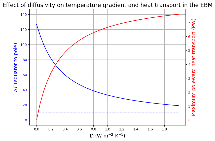
When , every latitude is in radiative equilibrium and the heat transport is zero. As we have already seen, this gives an equator-to-pole temperature gradient much too high.
When is large, the model is very efficient at moving heat poleward. The heat transport is large and the temperture gradient is weak.
The real climate seems to lie in a sweet spot in between these limits.
It looks like our fitting criteria are met reasonably well with W m K
Also, note that the global mean temperature (plotted in dashed blue) is completely insensitive to . Why do you think this is so?
We have chosen the following parameter values, which seems to give a reasonable fit to the observed annual mean temperature and energy budget:
There is one parameter left to choose: the heat capacity . We can’t use the annual mean energy budget and temperatures to guide this choice.
[Why?]
We will instead look at seasonally varying models in the next set of notes.
Credits
This notebook is part of The Climate Laboratory, an open-source textbook developed and maintained by Brian E. J. Rose, University at Albany.
It is licensed for free and open consumption under the Creative Commons Attribution 4.0 International (CC BY 4.0) license.
Development of these notes and the climlab software is partially supported by the National Science Foundation under award AGS-1455071 to Brian Rose. Any opinions, findings, conclusions or recommendations expressed here are mine and do not necessarily reflect the views of the National Science Foundation.
- Budyko, M. I. (1969). The effect of solar radiation variations on the climate of the Earth. Tellus, 21(5), 611–619.
- Sellers, W. D. (1969). A Global Climatic Model Based on the Energy Balance of the Earth-Atmosphere System. J. Appl. Meteor., 8(3), 392–400.