Due Wednesday September 11 2024 (at start of class, or submitted electronically via Brightspace before class)
Points per question: 5
Total points: 30
Question 1
(Problem 1.2 of the text) From Fig. 1.2, estimate the pressure at 10,000 m altitude, which is a typical cruising altitude for transcontinental airliners. About what fraction of the atmosphere’s mass is below you when you are at that altitude, given that average sea level pressure is 1013 hPa?
Question 2
(Problem 1.3 of the text) In Fig. 1.2a, the relationship between pressure and altitude is well approximated by a straight line. Because the pressure axis is logarithmic and the altitude axis is linear, this implies a mathematical relationship of the form:
where is the surface pressure and is called the scale height. From the figure, use the endpoints of the shaded area to estimate the average scale height.
Question 3
(Problem 1.5 of the text) On a particular day in Wisconsin, the pressure levels of 850 hPa and 700 hPa are found at altitudes of 1425 m and 2982 meters, respectively, and the corresponding temperatures are 3.8ºC and -2.9ºC. Determine the average lapse rate in degrees (to the nearest tenth) per kilometer.
Question 4
(Based on Problem 1.6 of the text)
For this exercise you will need to acess the University of Wyoming’s “Atmospheric Soundings” website at http://
Choose any region of the world and locate (but don’t click on) an upper air station of your choice. Also decide what date and time you are going to analyze. You may pick any date at all, for example:
the latest observation (today)
the date of an interesting weather event you remember
your last birthday
the day your dog was born
(a) Record the date, time, and station ID you will be using. Also provide a very brief justification (in words) for why you picked that station, date, and time.
(b) Select GIF: to 10 mb as the type of plot. Click on your chosen station and view the profile of temperature (heavy line on the right). Visually attempt to identify the tropopause, and estimate its height to the nearest 0.1 km from the height labels appearing just inside the left border of the plot. If the sounding terminates before reaching an obvious tropopause, then choose a different station or time for this exercise and note the change.
(c) Return to the main page, and this time select Text: List as the type of plot. Find the height and temperature at the surface level in the sounding. Also find the height and temperature at the 500 hPa level, if present; otherwise, use the highest available level. Use these data to determing the average lapse rate to the nearest 0.1 K/km between the two levels.
(d) Determine whether any inversions are found within the troposphere. If so, given their altitude and the magnitude of the temperature increase.
Question 5
(Problem 1.7 of the text) On a particular day in International Falls, Minnesota, the temperature is -4ºF and the wind speed is 10 knots. Determine the wind chill temperatures in degrees Fahrenheit, to the nearest degree.
Question 6
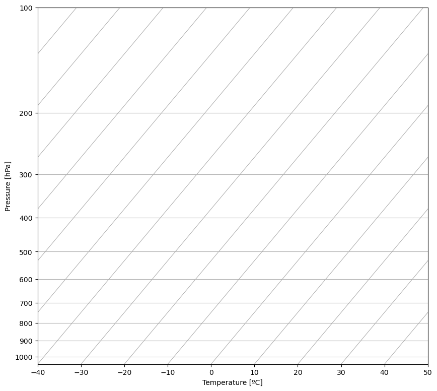
(Based on Problem 1.8 of the text) Use the attached skew-T chart below (which includes only isobars and isotherms) to plot by hand the following simplified temperature profile:
| pressure (hPa) | temperature (ºC) |
|---|---|
| 1014 | 20.0 |
| 980 | 20.3 |
| 878 | 17.6 |
| 830 | 19.0 |
| 500 | -11.5 |
| 400 | -25.1 |
| 267 | -46.1 |
| 213 | -49.1 |
| 142 | -67.5 |
| 100 | -72.7 |
You can ignore the code here! It’s just used to generate the blank chart that I want you to plot on by hand.
import matplotlib.pyplot as plt
from metpy.plots import SkewT
fig = plt.figure(figsize=(10, 14))
skew = SkewT(fig, rotation=40)
skew.ax.set_xlabel('Temperature [ºC]')
skew.ax.set_ylabel('Pressure [hPa]');