This notebook is part of The Climate Laboratory by Brian E. J. Rose, University at Albany.
1. The observed annual, global mean temperature profile
Let’s look again the observations of air temperature from the NCEP Reanalysis data we first encountered in the Radiation notes.
In this notebook we’ll define a function to create the Skew-T diagram, because later we are going to reuse it several times.
Click to expand code cells to see Python details
#  This code is used just to create the skew-T plot of global, annual mean air temperature
%matplotlib inline
import numpy as np
import matplotlib.pyplot as plt
import xarray as xr
from metpy.plots import SkewT
ncep_url = "http://www.esrl.noaa.gov/psd/thredds/dodsC/Datasets/ncep.reanalysis.derived/"
time_coder = xr.coders.CFDatetimeCoder(use_cftime=True)
ncep_air = xr.open_dataset( ncep_url + "pressure/air.mon.1981-2010.ltm.nc",
                           decode_times=time_coder)
#  Take global, annual average
coslat = np.cos(np.deg2rad(ncep_air.lat))
weight = coslat / coslat.mean(dim='lat')
Tglobal = (ncep_air.air * weight).mean(dim=('lat','lon','time'))
def make_skewT():
fig = plt.figure(figsize=(9, 9))
skew = SkewT(fig, rotation=30)
skew.plot(Tglobal.level, Tglobal, color='black', linestyle='-', linewidth=2, label='Observations')
skew.ax.set_ylim(1050, 10)
skew.ax.set_xlim(-90, 45)
# Add the relevant special lines
skew.plot_dry_adiabats(linewidth=0.5)
skew.plot_moist_adiabats(linewidth=0.5)
#skew.plot_mixing_lines()
skew.ax.legend()
skew.ax.set_xlabel('Temperature (degC)', fontsize=14)
skew.ax.set_ylabel('Pressure (hPa)', fontsize=14)
return skewskew = make_skewT()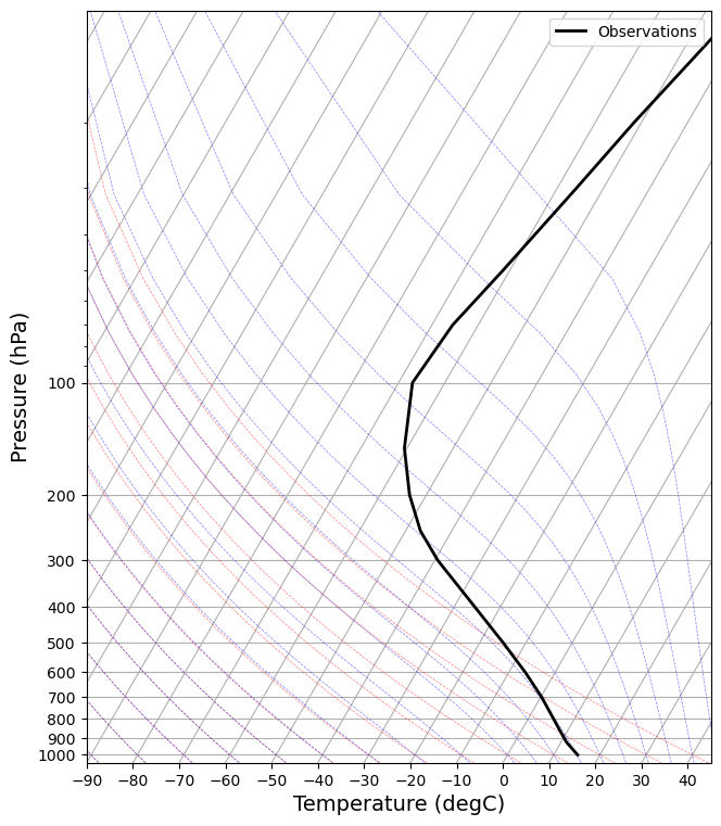
Here we are going to work with some detailed Single-Column Models to understand questions such as
- What physical factors actually determine this profile?
- Would the profile be different with different gases in the atmosphere?
- What are the relative roles of radiation and dynamics (i.e. motion!) in setting this profile?
We will start by ignoring all processes except radiation. We will calculate something called the radiative equilibrium temperature.
Models of radiative transfer slice up the atmospheric air column into a series of layer, and calculate the emission and absorption of radiation within each layer.
It’s really just a generalization of the model we already looked at:

The concept of radiative equilibrium means that we ignore all methods of heat exchange except for radiation, and ask what temperature profile would exist under that assumption?
We can answer that question by using a radiative transfer model to explicity compute the shortwave and longwave beams, and the warming/cooling of each layer associated with the radiative sources and sinks of energy.
Basically, we reach radiative equilibrium when energy is received and lost through radiation at the same rate in every layer.
Because of the complicated dependence of emission/absorption features on the wavelength of radiation and the different gases, the beam is divided up into many different pieces representing different parts of the electromagnetic spectrum.
We will not look explicitly at this complexity here, but we will use a model that represents these processes at the same level of detail we would in a GCM.
Radiation models in climlab
We’re now going to use climlab to run a complex radiation model, one that accounts for the spectral absorption properties of different gases.
climlab actually provides two different “GCM-level” radiation codes:
- The CAM3 radiation module from NCAR (essentially the same radiation code used in our CESM simulations)
- The RRTMG (Rapid Radiative Transfer Model) which is used in many current GCMs.
The links above take you to the online climlab documentation.
We’re going to use a model called the Rapid Radiative Transfer Model or RRTMG. This is a “serious” and widely-used radiation model, used in many comprehensive GCMs and Numerical Weather Prediction models.
climlab provides an easy-to-use Python wrapper for the RRTMG code.
Water vapor data
Before setting up the model, we need some water vapor data. Why? Because our model needs to know how much water vapor exists at each vertical level, since water vapor is a radiatively important gas.
We’re actually going to use the specific humidity field from our CESM control simulation. We’ll just take the global, time average of this data, and plot its vertical profile.
#  Load the model output as we have done before
cesm_data_path = "http://thredds.atmos.albany.edu:8080/thredds/dodsC/CESMA/"
atm_control = xr.open_dataset(cesm_data_path + "cpl_1850_f19/concatenated/cpl_1850_f19.cam.h0.nc")
#  The specific humidity is stored in the variable called Q in this dataset:
atm_control.QNow take the global, annual average of the specific humidity:
# Take global, annual average of the specific humidity
weight_factor = atm_control.gw / atm_control.gw.mean(dim='lat')
Qglobal = (atm_control.Q * weight_factor).mean(dim=('lat','lon','time'))
# Take a look at what we just calculated ... it should be one-dimensional (vertical levels)
QglobalAnd make a figure:
fig, ax = plt.subplots()
#  Multiply Qglobal by 1000 to put in units of grams water vapor per kg of air
ax.plot(Qglobal*1000., Qglobal.lev)
ax.invert_yaxis()
ax.set_ylabel('Pressure (hPa)')
ax.set_xlabel('Specific humidity (g/kg)')
ax.grid()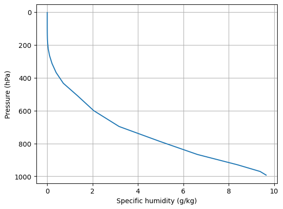
This shows a typical climatological humidity profile. Water vapor is a trace gas! But as we will see, it plays a very important role.
Based on this figure, where is most of the water vapor?
Create a single-column model on the same grid as this water vapor data:
Here we will create the grid and state variables (air and surface temperature) for our single-column model.
import climlab
#  Make a model on same vertical domain as the GCM
mystate = climlab.column_state(lev=Qglobal.lev, water_depth=2.5)
mystate
AttrDict({'Ts': Field([288.]), 'Tatm': Field([200. , 203.12, 206.24, 209.36, 212.48, 215.6 , 218.72, 221.84,
224.96, 228.08, 231.2 , 234.32, 237.44, 240.56, 243.68, 246.8 ,
249.92, 253.04, 256.16, 259.28, 262.4 , 265.52, 268.64, 271.76,
274.88, 278. ])})radmodel = climlab.radiation.RRTMG(name='Radiation (all gases)', # give our model a name!
state=mystate, # give our model an initial condition!
specific_humidity=Qglobal.values, # tell the model how much water vapor there is
albedo = 0.25, # this the SURFACE shortwave albedo
timestep = climlab.constants.seconds_per_day, # set the timestep to one day (measured in seconds)
)
radmodel<climlab.radiation.rrtm.rrtmg.RRTMG at 0x17fae7380>Explore the single-column model object
Look at a few interesting properties of the model we just created:
#  Here's the state dictionary we already created:
radmodel.state
AttrDict({'Ts': Field([288.]), 'Tatm': Field([200. , 203.12, 206.24, 209.36, 212.48, 215.6 , 218.72, 221.84,
224.96, 228.08, 231.2 , 234.32, 237.44, 240.56, 243.68, 246.8 ,
249.92, 253.04, 256.16, 259.28, 262.4 , 265.52, 268.64, 271.76,
274.88, 278. ])})# Here are the pressure levels in hPa
radmodel.levarray([ 3.544638 , 7.3888135, 13.967214 , 23.944625 , 37.23029 ,
53.114605 , 70.05915 , 85.439115 , 100.514695 , 118.250335 ,
139.115395 , 163.66207 , 192.539935 , 226.513265 , 266.481155 ,
313.501265 , 368.81798 , 433.895225 , 510.455255 , 600.5242 ,
696.79629 , 787.70206 , 867.16076 , 929.648875 , 970.55483 ,
992.5561 ])There is a dictionary called absorber_vmr that holds the volume mixing ratio of all the radiatively active gases in the column:
radmodel.absorber_vmr{'CO2': 0.000348,
'CH4': 1.65e-06,
'N2O': 3.06e-07,
'O2': 0.21,
'CFC11': 0.0,
'CFC12': 0.0,
'CFC22': 0.0,
'CCL4': 0.0,
'O3': array([7.52507018e-06, 8.51545793e-06, 7.87041289e-06, 5.59601020e-06,
3.46128454e-06, 2.02820936e-06, 1.13263102e-06, 7.30182697e-07,
5.27326553e-07, 3.83940962e-07, 2.82227214e-07, 2.12188506e-07,
1.62569291e-07, 1.17991442e-07, 8.23582543e-08, 6.25738219e-08,
5.34457156e-08, 4.72688637e-08, 4.23614749e-08, 3.91392482e-08,
3.56025264e-08, 3.12026770e-08, 2.73165152e-08, 2.47190016e-08,
2.30518624e-08, 2.22005071e-08])}Most are just a single number because they are assumed to be well mixed in the atmosphere.
The exception is ozone, which has a vertical structure taken from observations. Let’s plot it
#  E.g. the CO2 content (a well-mixed gas) in parts per million
radmodel.absorber_vmr['CO2'] * 1E6348.0Python exercise: plot the ozone profile
Make a simple plot showing the vertical structure of ozone, similar to the specific humidity plot we just made above.
# here is the data you need for the plot, as a plain numpy arrays:
print(radmodel.lev)
print(radmodel.absorber_vmr['O3'])
[ 3.544638 7.3888135 13.967214 23.944625 37.23029 53.114605
70.05915 85.439115 100.514695 118.250335 139.115395 163.66207
192.539935 226.513265 266.481155 313.501265 368.81798 433.895225
510.455255 600.5242 696.79629 787.70206 867.16076 929.648875
970.55483 992.5561 ]
[7.52507018e-06 8.51545793e-06 7.87041289e-06 5.59601020e-06
3.46128454e-06 2.02820936e-06 1.13263102e-06 7.30182697e-07
5.27326553e-07 3.83940962e-07 2.82227214e-07 2.12188506e-07
1.62569291e-07 1.17991442e-07 8.23582543e-08 6.25738219e-08
5.34457156e-08 4.72688637e-08 4.23614749e-08 3.91392482e-08
3.56025264e-08 3.12026770e-08 2.73165152e-08 2.47190016e-08
2.30518624e-08 2.22005071e-08]
The other radiatively important gas is of course water vapor, which is stored separately in the specific_humidity attribute:
#  specific humidity in kg/kg, on the same pressure axis
radmodel.specific_humidity
array([2.16104904e-06, 2.15879387e-06, 2.15121262e-06, 2.13630949e-06,
2.12163684e-06, 2.11168002e-06, 2.09396914e-06, 2.10589390e-06,
2.42166155e-06, 3.12595653e-06, 5.01369691e-06, 9.60746488e-06,
2.08907654e-05, 4.78823747e-05, 1.05492451e-04, 2.11889055e-04,
3.94176751e-04, 7.10734458e-04, 1.34192099e-03, 2.05153261e-03,
3.16844784e-03, 4.96883408e-03, 6.62218037e-03, 8.38350326e-03,
9.38620899e-03, 9.65030544e-03])The RRTMG radiation model has lots of different input parameters
For details you can look at the documentation
for item in radmodel.input:
    print(item)
specific_humidity
absorber_vmr
cldfrac
clwp
ciwp
r_liq
r_ice
emissivity
S0
coszen
irradiance_factor
aldif
aldir
asdif
asdir
icld
irng
idrv
permuteseed_sw
permuteseed_lw
dyofyr
inflgsw
inflglw
iceflgsw
iceflglw
liqflgsw
liqflglw
tauc_sw
tauc_lw
ssac_sw
asmc_sw
fsfc_sw
tauaer_sw
ssaaer_sw
asmaer_sw
ecaer_sw
tauaer_lw
isolvar
indsolvar
bndsolvar
solcycfrac
Many of the parameters control the radiative effects of clouds.
But here we should note that the model is initialized with no clouds at all:
#  This is the fractional area covered by clouds in our column:
radmodel.cldfrac0.0Step the model forward in time!
Here are the current temperatures (initial condition):
radmodel.TsField([288.])radmodel.TatmField([200. , 203.12, 206.24, 209.36, 212.48, 215.6 , 218.72, 221.84,
224.96, 228.08, 231.2 , 234.32, 237.44, 240.56, 243.68, 246.8 ,
249.92, 253.04, 256.16, 259.28, 262.4 , 265.52, 268.64, 271.76,
274.88, 278. ])Now let’s take a single timestep:
radmodel.step_forward()radmodel.TsField([288.57727148])The surface got warmer!
Let’s take a look at all the diagnostic information that was generated during that timestep:
Diagnostic variables in our single-column model
Every climlab model has a diagnostics dictionary. Here we are going to check it out as an xarray dataset:
climlab.to_xarray(radmodel.diagnostics)The main “job” of a radiative transfer model it to calculate the shortwave and longwave fluxes up and down between each model layer.
For example:
climlab.to_xarray(radmodel.LW_flux_up)These are upward longwave fluxes in W/m2.
Why are there 27 data points, when the model has 26 pressure levels?
radmodel.levarray([ 3.544638 , 7.3888135, 13.967214 , 23.944625 , 37.23029 ,
53.114605 , 70.05915 , 85.439115 , 100.514695 , 118.250335 ,
139.115395 , 163.66207 , 192.539935 , 226.513265 , 266.481155 ,
313.501265 , 368.81798 , 433.895225 , 510.455255 , 600.5242 ,
696.79629 , 787.70206 , 867.16076 , 929.648875 , 970.55483 ,
992.5561 ])radmodel.lev_boundsarray([ 0. , 5.46672575, 10.67801375, 18.9559195 ,
30.5874575 , 45.1724475 , 61.5868775 , 77.7491325 ,
92.976905 , 109.382515 , 128.682865 , 151.3887325 ,
178.1010025 , 209.5266 , 246.49721 , 289.99121 ,
341.1596225 , 401.3566025 , 472.17524 , 555.4897275 ,
648.660245 , 742.249175 , 827.43141 , 898.4048175 ,
950.1018525 , 981.555465 , 1000. ])The last element of the flux array represents the upward flux from the surface to the first level:
radmodel.LW_flux_up[-1]np.float64(390.0990181032836)The value is about 390 W m.
Why?
sigma = 5.67E-8
sigma * 288**4390.0793946112The surface temperature was initialized at 288 K, and the surface is treated as very close to a blackbody in the model.
What about the flux from the top layer out to space?
Two ways to access this information:
radmodel.LW_flux_up[0]np.float64(251.01459805907507)radmodel.OLRField([251.01459806])Of course there is a whole other set of fluxes for the shortwave radiation.
One diagnostic we will often want to look at is the net energy budget at the top of the atmosphere:
radmodel.ASR - radmodel.OLRField([3.76767763])Is the model gaining or losing energy?
Integrate out to equilibrium
Here I want to step forward in time until the model is very close to energy balance.
We can use a while loop, conditional on the top-of-atmosphere imbalance:
while np.abs(radmodel.ASR - radmodel.OLR) > 0.01:
    radmodel.step_forward()
Check the energy budget again:
#  Check the energy budget again
radmodel.ASR - radmodel.OLRField([0.00988074])Indeed, the imbalance is now small.
Compare the radiative equilibrium temperature to observations
Here’s a helper function we’ll use to add model temperature profiles to our skew-T plot:
def add_profile(skew, model, linestyle='-', color=None):
    line = skew.plot(model.lev, model.Tatm - climlab.constants.tempCtoK,
             label=model.name, linewidth=2)[0]
    skew.plot(1000, model.Ts - climlab.constants.tempCtoK, 'o',
              markersize=8, color=line.get_color())
    skew.ax.legend()
skew = make_skewT()
add_profile(skew, radmodel)
skew.ax.set_title('Pure radiative equilibrium', fontsize=18);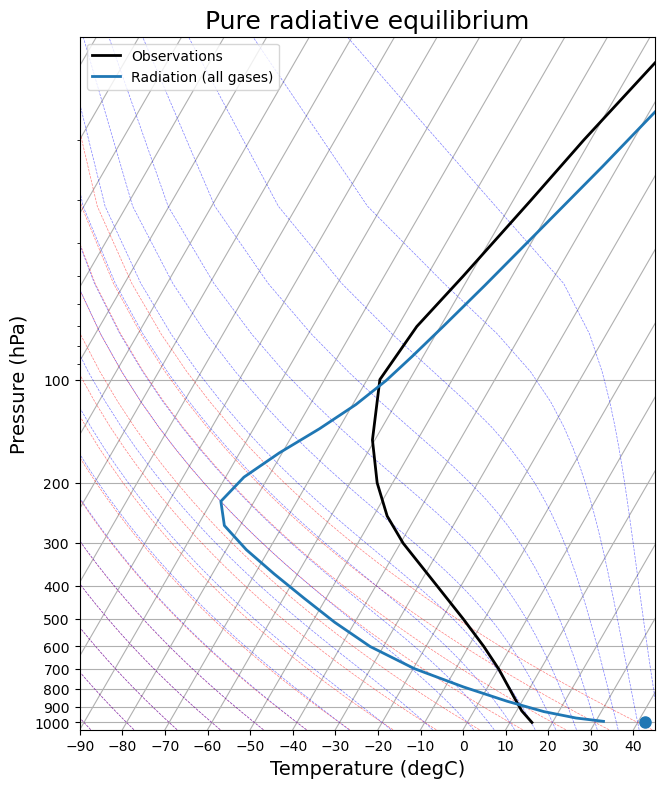
What do you think about this model -- data comparison?
Models are for experimenting and playing with!
We have just built a single-column radiation model with several different absorbing gases. We can learn about their effects by taking them away.
Radiative equilibrium without water vapor
# Make an exact clone of our existing model
radmodel_noH2O = climlab.process_like(radmodel)
radmodel_noH2O.name = 'Radiation (no H2O)'
radmodel_noH2O
<climlab.radiation.rrtm.rrtmg.RRTMG at 0x17fd739d0># Here is the water vapor profile we started with
radmodel_noH2O.specific_humidityarray([2.16104904e-06, 2.15879387e-06, 2.15121262e-06, 2.13630949e-06,
2.12163684e-06, 2.11168002e-06, 2.09396914e-06, 2.10589390e-06,
2.42166155e-06, 3.12595653e-06, 5.01369691e-06, 9.60746488e-06,
2.08907654e-05, 4.78823747e-05, 1.05492451e-04, 2.11889055e-04,
3.94176751e-04, 7.10734458e-04, 1.34192099e-03, 2.05153261e-03,
3.16844784e-03, 4.96883408e-03, 6.62218037e-03, 8.38350326e-03,
9.38620899e-03, 9.65030544e-03])Now get rid of the water entirely!
radmodel_noH2O.specific_humidity *= 0.radmodel_noH2O.specific_humidityarray([0., 0., 0., 0., 0., 0., 0., 0., 0., 0., 0., 0., 0., 0., 0., 0., 0.,
0., 0., 0., 0., 0., 0., 0., 0., 0.])And run this new model forward to equilibrium:
#  it's useful to take a single step first before starting the while loop
#   because the diagnostics won't get updated
#  (and thus show the effects of removing water vapor)
#  until we take a step forward
radmodel_noH2O.step_forward()
while np.abs(radmodel_noH2O.ASR - radmodel_noH2O.OLR) > 0.01:
    radmodel_noH2O.step_forward()
radmodel_noH2O.ASR - radmodel_noH2O.OLRField([-0.00999903])skew = make_skewT()
for model in [radmodel, radmodel_noH2O]:
add_profile(skew, model)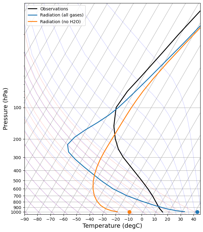
What do you think you can learn from this about the radiative role of water vapor?
Exercise: radiative equilibrium without ozone
Following the steps above, make another model, but this time instead of removing the water vapor, remove the ozone!
Make another skew-T plot comparing all three model results.
If you have time, try a third case in which you remove both the water vapor and the ozone!
- We used the RRTMG radiation model with prescribed profiles of absorbing gases to calculate pure radiative equilibrium temperature profiles.
- Radiative Equilibrium means the temperatures that the surface and air column would have if radiation was the only physical process that could transfer energy between levels.
- We computed several different radiative equilibrium profiles, with and without key absorbing gases
- The profile without water vapor is much colder at surface and lower troposphere, but about the same in the stratosphere
- The profile without ozone is much colder in the stratosphere, but about the same near the surface.
- In fact there really isn’t a stratosphere at all without ozone! The temperature is nearly isothermal in the upper atmosphere in that profile.
However the really key takeaway message is that none of these radiative equilibrium profiles look much like the observations in the troposphere.
This strongly suggests that other physical processes (aside from radiation) are important in determining the observed temperature profile.
Plotting on the skew-T diagram makes it clear that all the radiative equilibrium profiles are statically unstable near the surface.
The next step is therefore to look at the effects of convective mixing on the temperatures of the surface and lower troposphere.
Credits
This notebook is part of The Climate Laboratory, an open-source textbook developed and maintained by Brian E. J. Rose, University at Albany.
It is licensed for free and open consumption under the Creative Commons Attribution 4.0 International (CC BY 4.0) license.
Development of these notes and the climlab software is partially supported by the National Science Foundation under award AGS-1455071 to Brian Rose. Any opinions, findings, conclusions or recommendations expressed here are mine and do not necessarily reflect the views of the National Science Foundation.