Radiative-Convective Equilibrium - The Climate Laboratory

This notebook is part of The Climate Laboratory by Brian E. J. Rose, University at Albany.

1. Recap of radiative equilibrium results¶

Here we summarize results we generated in the Lecture on radiative equilibrium.

%matplotlib inline
import numpy as np
import matplotlib.pyplot as plt
import xarray as xr
from metpy.plots import SkewT
#  This code is used just to create the skew-T plot of global, annual mean air temperature
ncep_url = "http://www.esrl.noaa.gov/psd/thredds/dodsC/Datasets/ncep.reanalysis.derived/"
time_coder = xr.coders.CFDatetimeCoder(use_cftime=True)
ncep_air = xr.open_dataset( ncep_url + "pressure/air.mon.1981-2010.ltm.nc", decode_times=time_coder)
#  Take global, annual average 
coslat = np.cos(np.deg2rad(ncep_air.lat))
weight = coslat / coslat.mean(dim='lat')
Tglobal = (ncep_air.air * weight).mean(dim=('lat','lon','time'))
#  Resuable function to plot the temperature data on a Skew-T chart
def make_skewT():
    fig = plt.figure(figsize=(9, 9))
    skew = SkewT(fig, rotation=30)
    skew.plot(Tglobal.level, Tglobal, color='black', linestyle='-', linewidth=2, label='Observations')
    skew.ax.set_ylim(1050, 10)
    skew.ax.set_xlim(-90, 45)
    # Add the relevant special lines
    skew.plot_dry_adiabats(linewidth=0.5)
    skew.plot_moist_adiabats(linewidth=0.5)
    #skew.plot_mixing_lines()
    skew.ax.legend()
    skew.ax.set_xlabel('Temperature (degC)', fontsize=14)
    skew.ax.set_ylabel('Pressure (hPa)', fontsize=14)
    return skew
#  and a function to add extra profiles to this chart
def add_profile(skew, model, linestyle='-', color=None):
    line = skew.plot(model.lev, model.Tatm - climlab.constants.tempCtoK,
             label=model.name, linewidth=2)[0]
    skew.plot(1000, model.Ts - climlab.constants.tempCtoK, 'o', 
              markersize=8, color=line.get_color())
    skew.ax.legend()

# Get the water vapor data from CESM output
cesm_data_path = "http://thredds.atmos.albany.edu:8080/thredds/dodsC/CESMA/"
# For better performance if you can access the roselab_rit filesystem (e.g. from JupyterHub)
# cesm_data_path = "/roselab_rit/cesm_archive/"
atm_control = xr.open_dataset(cesm_data_path + "cpl_1850_f19/concatenated/cpl_1850_f19.cam.h0.nc")
# Take global, annual average of the specific humidity
weight_factor = atm_control.gw / atm_control.gw.mean(dim='lat')
Qglobal = (atm_control.Q * weight_factor).mean(dim=('lat','lon','time'))
#  Create the single-column model domain
import climlab
#  Make a model on same vertical domain as the GCM
mystate = climlab.column_state(lev=Qglobal.lev, water_depth=2.5)
#  Create the model itself -- radiation only!
rad = climlab.radiation.RRTMG(name='Radiation (all gases)',  # give our model a name!
                              state=mystate,   # give our model an initial condition!
                              specific_humidity=Qglobal.values,  # tell the model how much water vapor there is
                              albedo = 0.25,  # this the SURFACE shortwave albedo
                              timestep = climlab.constants.seconds_per_day,  # set the timestep to one day (measured in seconds)
                             )

#  remove ozone
rad_noO3 = climlab.process_like(rad)
rad_noO3.absorber_vmr['O3'] *= 0.
rad_noO3.name = 'no O3'
#  remove water vapor
rad_noH2O = climlab.process_like(rad)
rad_noH2O.specific_humidity *= 0.
rad_noH2O.name = 'no H2O'
#  remove both
rad_noO3_noH2O = climlab.process_like(rad_noO3)
rad_noO3_noH2O.specific_humidity *= 0.
rad_noO3_noH2O.name = 'no O3, no H2O'
#  put all models together in a list
rad_models = [rad, rad_noO3, rad_noH2O, rad_noO3_noH2O]

#  Loop through the models and integrate each one out to equilibrium
for model in rad_models:
    for n in range(100):
        model.step_forward()
    while (np.abs(model.ASR-model.OLR)>0.01):
        model.step_forward()
        
# Plot all the results
skew = make_skewT()
for model in rad_models:
    add_profile(skew, model)
skew.ax.set_title('Pure radiative equilibrium', fontsize=18);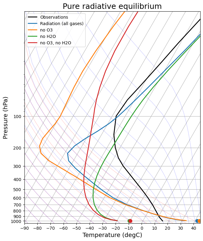

As we have already discussed, none of these profiles really looks anything like the observations in the troposphere. This strongly suggests that other physical processes (aside from radiation) are important in determining the observed temperature profile.

Plotting on the skew-T diagram makes it clear that all the radiative equilibrium profiles are statically unstable near the surface.

So we’re now going to add a representation of the effects of convective mixing to the single-column model.

2. Building a radiative-convection model in climlab¶

To make a Radiative-Convective model, we just take a radiation model and couple it to a convection model!

The “convection” model we’re going to use here is available as

climlab.convection.ConvectiveAdjustment

It is a simple process that looks for lapse rates exceeding a critical threshold and performs an instantaneous adjustment that mixes temperatures to the critical lapse rate while conserving energy.

This is a parameterization of the complex, rapid mixing processes that actually occur in an unstable air column!

Here is some code to put this model together in climlab:

#  Make a model on same vertical domain as the GCM
mystate = climlab.column_state(lev=Qglobal.lev, water_depth=2.5)
#  Build the radiation model -- just like we already did
rad = climlab.radiation.RRTMG(name='Radiation (net)',
                              state=mystate, 
                              specific_humidity=Qglobal.values,
                              timestep = climlab.constants.seconds_per_day,
                              albedo = 0.25,  # surface albedo, tuned to give reasonable ASR for reference cloud-free model
                             )
#  Now create the convection model
conv = climlab.convection.ConvectiveAdjustment(name='Convection',
                                               state=mystate,
                                               adj_lapse_rate=6.5, # this is the key parameter! We'll discuss below
                                               timestep=rad.timestep,  # same timestep!
                                              )
#  Here is where we build the model by coupling together the two components
rcm = climlab.couple([rad, conv], name='Radiative-Convective Model')

rcm

<climlab.process.time_dependent_process.TimeDependentProcess at 0x17dab1940>

3. Adjustment toward radiative-convective equilibrium¶

Adjustment from isothermal initial conditions¶

To get some insight into the interaction between radiation and convection, it’s useful to look at the adjustment process from a non-equilibrium initial condition.

Let’s make an animation!

The code below is complicated but it is mostly for generating the animation. Focus on the results, not the code here.

#  Some imports needed to make and display animations
from IPython.display import HTML
from matplotlib import animation

def get_tendencies(model):
    '''Pack all the subprocess tendencies into xarray.Datasets
    and convert to units of K / day'''
    tendencies_atm = xr.Dataset()
    tendencies_sfc = xr.Dataset()
    for name, proc, top_proc in climlab.utils.walk.walk_processes(model, topname='Total', topdown=False):
        tendencies_atm[name] = proc.tendencies['Tatm'].to_xarray()
        tendencies_sfc[name] = proc.tendencies['Ts'].to_xarray()
    for tend in [tendencies_atm, tendencies_sfc]:
        #  convert to K / day
        tend *= climlab.constants.seconds_per_day
    return tendencies_atm, tendencies_sfc

def initial_figure(model):
    fig = plt.figure(figsize=(14,6))
    lines = []
    
    skew = SkewT(fig, subplot=(1,2,1), rotation=30)
    #  plot the observations
    skew.plot(Tglobal.level, Tglobal, color='black', linestyle='-', linewidth=2, label='Observations')    
    lines.append(skew.plot(model.lev, model.Tatm - climlab.constants.tempCtoK, 
              linestyle='-', linewidth=2, color='C0', label='RC model (all gases)')[0])
    skew.ax.legend()
    skew.ax.set_ylim(1050, 10)
    skew.ax.set_xlim(-60, 75)
    # Add the relevant special lines
    skew.plot_dry_adiabats(linewidth=0.5)
    skew.plot_moist_adiabats(linewidth=0.5)
    skew.ax.set_xlabel('Temperature (°C)', fontsize=14)
    skew.ax.set_ylabel('Pressure (hPa)', fontsize=14)
    lines.append(skew.plot(1000, model.Ts - climlab.constants.tempCtoK, 'o', 
                  markersize=8, color='C0', )[0])

    ax = fig.add_subplot(1,2,2, sharey=skew.ax)
    ax.set_ylim(1050, 10)
    ax.set_xlim(-8,8)
    ax.grid()
    ax.set_xlabel(r'Temperature tendency (°C day$^{-1}$)', fontsize=14)

    color_cycle=['g','b','r','y','k']
    #color_cycle=['y', 'r', 'b', 'g', 'k']
    tendencies_atm, tendencies_sfc = get_tendencies(rcm)
    for i, name in enumerate(tendencies_atm.data_vars):
        lines.append(ax.plot(tendencies_atm[name], model.lev, label=name, color=color_cycle[i])[0])
    for i, name in enumerate(tendencies_sfc.data_vars):
        lines.append(ax.plot(tendencies_sfc[name], 1000, 'o', markersize=8, color=color_cycle[i])[0])
    ax.legend(loc='center right');
    lines.append(skew.ax.text(-100, 50, 'Day {}'.format(int(model.time['days_elapsed'])), fontsize=12)) 
    return fig, lines

def animate(day, model, lines):
    lines[0].set_xdata(np.array(model.Tatm)-climlab.constants.tempCtoK)
    lines[1].set_xdata(np.array(model.Ts)-climlab.constants.tempCtoK)
    #lines[2].set_xdata(np.array(model.q)*1E3)
    tendencies_atm, tendencies_sfc = get_tendencies(model)
    for i, name in enumerate(tendencies_atm.data_vars):
        lines[2+i].set_xdata(tendencies_atm[name])
    for i, name in enumerate(tendencies_sfc.data_vars):
        lines[2+5+i].set_xdata(tendencies_sfc[name])
    lines[-1].set_text('Day {}'.format(int(model.time['days_elapsed'])))
    # This is kind of a hack, but without it the initial frame doesn't appear
    if day != 0:
        model.step_forward()
    return lines

We are going to start from an isothermal initial state, and let the model drift toward equilibrium.

#  Start from isothermal state
rcm.state.Tatm[:] = rcm.state.Ts
#  Call the diagnostics once for initial plotting
rcm.compute_diagnostics()
#  Plot initial data
fig, lines = initial_figure(rcm)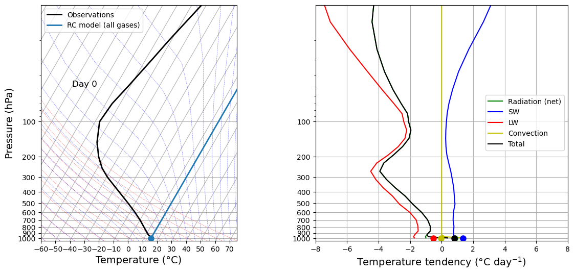

Notice several things here:

The initial profile is isothermal at 15ºC. This is an arbitrary choice we made.
The initial tendency from convection is zero everywhere. Why?
Shortwave radiation tends to warm everywhere. Why?
Longwave radiation tends to cool everywhere. The cooling is very strong especially aloft. Why?
The total tendency (black) is warming at the surface and cooling in the atmosphere. What should happen next? What are the implications for convective instability?

Now let’s look at how the model actually adjusts:

#  This is where we make a loop over many timesteps and create an animation in the notebook
ani = animation.FuncAnimation(fig, animate, 150, fargs=(rcm, lines))
HTML(ani.to_html5_video())

Discuss.

What if instead we start out from pure Radiative equilibrium?¶

This will represent the effect of a sudden “switching on” of convective processes.

#  Here we take JUST THE RADIATION COMPONENT of the full model and run it out to (near) equilibrium
#  This is just to get the initial condition for our animation
for n in range(1000):
    rcm.subprocess['Radiation (net)'].step_forward()

#  Call the diagnostics once for initial plotting
rcm.compute_diagnostics()
#  Plot initial data
fig, lines = initial_figure(rcm)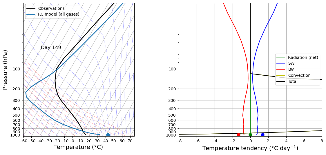

#  This is where we make a loop over many timesteps and create an animation in the notebook
ani = animation.FuncAnimation(fig, animate, 100, fargs=(rcm, lines))
HTML(ani.to_html5_video())

This animation is not as exciting because the instability is destroyed immediately in the first timestep!

That is because the ConvectiveAdjustment process operates instantaneously whenever there is any instability. It is a parameterization taking advantage of the fact that, in nature, convection processes are fast compared to radiative processes.

But notice that the final state is pretty much the same as in the first animation.

The column tends toward the same equilibrium state regardless of where it starts.

4. Compare Radiative- and Radiative-Convective Equilibrium¶

Let’s repeat our experiment with removing certain absorbing gases from the model, but use the Radiative-Convective model.

#  Make a model on same vertical domain as the GCM
mystate = climlab.column_state(lev=Qglobal.lev, water_depth=2.5)

rad = climlab.radiation.RRTMG(name='all gases',
                              state=mystate, 
                              specific_humidity=Qglobal.values,
                              timestep = climlab.constants.seconds_per_day,
                              albedo = 0.25,  # tuned to give reasonable ASR for reference cloud-free model
                             )
#  remove ozone
rad_noO3 = climlab.process_like(rad)
rad_noO3.absorber_vmr['O3'] *= 0.
rad_noO3.name = 'no O3'
#  remove water vapor
rad_noH2O = climlab.process_like(rad)
rad_noH2O.specific_humidity *= 0.
rad_noH2O.name = 'no H2O'
#  remove both
rad_noO3_noH2O = climlab.process_like(rad_noO3)
rad_noO3_noH2O.specific_humidity *= 0.
rad_noO3_noH2O.name = 'no O3, no H2O'
#  put all models together in a list
rad_models = [rad, rad_noO3, rad_noH2O, rad_noO3_noH2O]

rc_models = []
for r in rad_models:
    newrad = climlab.process_like(r)
    conv = climlab.convection.ConvectiveAdjustment(name='Convective Adjustment',
                                               state=newrad.state,
                                               adj_lapse_rate=6.5,  # the key parameter in the convection model!
                                               timestep=newrad.timestep,)
    rc = climlab.couple([newrad, conv], name=newrad.name)
    rc_models.append(rc)

for model in rad_models:
    for n in range(100):
        model.step_forward()
    while (np.abs(model.ASR-model.OLR)>0.01):
        model.step_forward()    
    
for model in rc_models:
    for n in range(100):
        model.step_forward()
    while (np.abs(model.ASR-model.OLR)>0.01):
        model.step_forward()

skew = make_skewT()
for model in rad_models:
    add_profile(skew, model)
skew.ax.set_title('Pure radiative equilibrium', fontsize=18);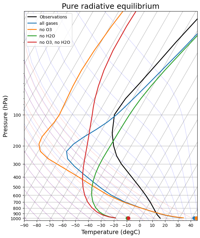

skew2 = make_skewT()
for model in rc_models:
    add_profile(skew2, model)
skew2.ax.set_title('Radiative-convective equilibrium', fontsize=18);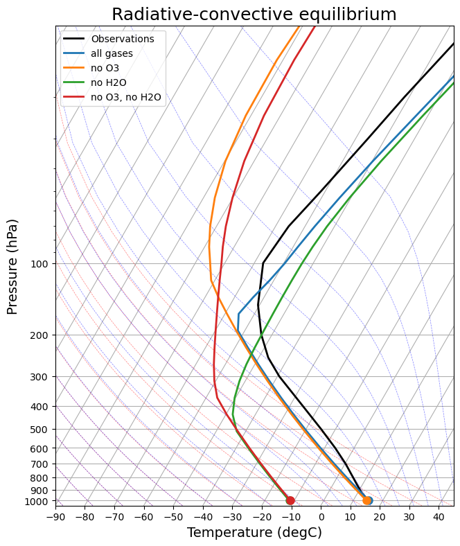

Lots to discuss here.

The overall message is that equilibrium temperature profile results from a competition between radiation and convection. Essentially:

Radiation is always trying to push temperatures toward radiative equilibrium, which means
- warm surface
- cold troposphere
Convection cools the surface and warms the troposphere
The troposphere can be defined here as the layer over which convection is active.
This is true whether or not we have the radiative effects of water vapor.
When we remove the water vapor (and its warming greenhouse effect), the surface temperature becomes much colder and the troposphere is much shallower -- but it is still there.

5. The role of the critical lapse rate¶

What have we done above¶

These calculations all used a critical lapse rate of 6.5 K / km, which is a reasonable approximation to observations.

We set this with the input argument

adj_lapse_rate

to the ConvectiveAdjustment process.

The idea is that we are trying to represent the statistical effects of many episodes of moist convection.

An air column that is perfectly neutral to moist instability would follow the blue moist adiabats on the skew-T diagrams.

We can force the model to behave this way by setting

adj_lapse_rate = 'pseudoadiabat'

However the real atmosphere, on average, does not exactly follow these adiabats for several reasons:

the slope of the moist adiabat depends strongly on temperature (as we can see on these diagrams)
We are looking at temperatures averaged over the whole planet, including regions that are warm and moist, warm and dry, and cold.
Heat fluxes by mid-latitude eddies play an important role in stabilizing the extra-tropical atmosphere.

So here we sweep all this complexity under the rug and just choose a single critical lapse rate for our convective adjustment model.

But this is a parameter that is uncertain and could be interesting to explore.

Python exercise: change the critical lapse rate¶

Repeat the whole series of calculations for the different combinations of absorbing gases above, but with different critical lapse rates:

adj_lapse_rate = 9.8 (in K/km, the dry adiabatic lapse rate, suitable for an atmosphere where condensation does not impact the buoyancy of air parcels)
adj_lapse_rate = 'pseudoadiabat' (more suitable for the tropical atmosphere)

6. Summary of radiative-convection equilibrium results¶

We noted that pure radiative equilibrium is not a good model for the observed temperature profile.
An air column in radiative equilibrium has a warm surface and cold troposphere.
In reality this would tend to become unstable and cause vertical mixing.

To account for this shortcoming of the radiation model, we coupled our single-column radiation model (using the RRTMG radiation model) to a simple convection model.

The ConvectiveAdjustment model instantly mixes out any profiles where the lapse rate exceeds some critical threshold value.
This critical lapse rate is the tunable parameter in our combined Radiative-Convective Model or RCM.
Using a value of 6.5 K / km and realistic gas profiles gives a reasonable (not perfect) fit to the observed air temperatures.
The RCM represents the “tug-of-war” between radiation (trying to warm the surface and cool the troposphere) and convection (cool the surface and warm the troposphere).
The convectively mixed layer extends up to near the top of the troposphere.

Our experiments with removing certain absorbing gases show something interesting: the height of the tropopause (boundary bewteen troposphere and stratosphere) changes when we remove absorbers. Warmer columns also appear to have higher tropopause.

Now that we know how to build and use this RCM, we’ll be able to use to study some climate change processes in more detail.

Credits¶

This notebook is part of The Climate Laboratory, an open-source textbook developed and maintained by Brian E. J. Rose, University at Albany.

It is licensed for free and open consumption under the Creative Commons Attribution 4.0 International (CC BY 4.0) license.

Development of these notes and the climlab software is partially supported by the National Science Foundation under award AGS-1455071 to Brian Rose. Any opinions, findings, conclusions or recommendations expressed here are mine and do not necessarily reflect the views of the National Science Foundation.