1. Top-of-Atmosphere Radiation Budget and Meridional Energy Transport#
Overview and goals#
In this assignment you will use data from the CERES-EBAF product as we did in the first set of lecture notes.
This assigment has several goals:
Build skills in loading and manipulating datasets
Compute global averages
Verify the data against a published result
Learn the basic method for calculating meridional transport from local imbalances
Apply that method to compute meridional energy transport from the CERES-EBAF data
Instructions#
In a local copy of this notebook add your answers in additional cells.
Complete both problems below.
Remember to set your cell types to
Markdownfor text, andCodefor Python code!Include comments in your code to explain your method as necessary.
Remember to actually answer the questions. Written answers are required (not just code and figures!)
Submit your solutions in a single Jupyter notebook that contains your text, your code, and your figures.
Make sure that your notebook runs cleanly without errors:
Save your notebook
From the
Kernelmenu, selectRestart & Run AllDid the notebook run from start to finish without error and produce the expected output?
If yes, save again and submit your notebook file
If no, fix the errors and try again.
Problem 1: global, annual mean energy budgets#
Consider the first figure in our lecture notes from Stephens et al. [2012] and reproduced again here:
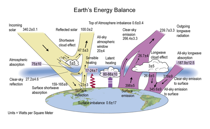
Your task here is simply to reproduce as many of the values shown in this figure as you can from the CERES-EBAF dataset. Remember that these values all represent long-term time averages and global averages, and that global averages must be properly weighted to account for the area of grid cells. If you’re looking for help on the area weighting, check out this short lesson from the xarray docs.
Please include all your code here in the notebook, but also summarize your results clearly. This might be as a table, or formatted output from Python code, or any other way which is easy to read and compare against the values in the figure.
Comment on any interesting similarities or differences that you find between your results and the values in the figure.
To get you started, here is the same code we used in the lecture notes to access the CERES-EBAF data:
import xarray as xr

ceres_path = '/nfs/roselab_rit/data/CERES_EBAF/'
ceres_filename_prefix = 'CERES_EBAF_Ed4.1_Subset_'
ceres_files = [ceres_path + ceres_filename_prefix + '200003-201412.nc',
               ceres_path + ceres_filename_prefix + '201501-202202.nc',]

ceres = xr.open_mfdataset(ceres_files)
ceres
<xarray.Dataset>
Dimensions:                      (lon: 360, lat: 180, time: 264)
Coordinates:
  * lon                          (lon) float32 0.5 1.5 2.5 ... 357.5 358.5 359.5
  * lat                          (lat) float32 -89.5 -88.5 -87.5 ... 88.5 89.5
  * time                         (time) datetime64[ns] 2000-03-15 ... 2022-02-15
Data variables: (12/41)
    toa_sw_all_mon               (time, lat, lon) float32 dask.array<chunksize=(178, 180, 360), meta=np.ndarray>
    toa_lw_all_mon               (time, lat, lon) float32 dask.array<chunksize=(178, 180, 360), meta=np.ndarray>
    toa_net_all_mon              (time, lat, lon) float32 dask.array<chunksize=(178, 180, 360), meta=np.ndarray>
    toa_sw_clr_c_mon             (time, lat, lon) float32 dask.array<chunksize=(178, 180, 360), meta=np.ndarray>
    toa_lw_clr_c_mon             (time, lat, lon) float32 dask.array<chunksize=(178, 180, 360), meta=np.ndarray>
    toa_net_clr_c_mon            (time, lat, lon) float32 dask.array<chunksize=(178, 180, 360), meta=np.ndarray>
    ...                           ...
    sfc_net_tot_all_mon          (time, lat, lon) float32 dask.array<chunksize=(178, 180, 360), meta=np.ndarray>
    sfc_net_tot_clr_c_mon        (time, lat, lon) float32 dask.array<chunksize=(178, 180, 360), meta=np.ndarray>
    sfc_net_tot_clr_t_mon        (time, lat, lon) float32 dask.array<chunksize=(178, 180, 360), meta=np.ndarray>
    sfc_cre_net_sw_mon           (time, lat, lon) float32 dask.array<chunksize=(178, 180, 360), meta=np.ndarray>
    sfc_cre_net_lw_mon           (time, lat, lon) float32 dask.array<chunksize=(178, 180, 360), meta=np.ndarray>
    sfc_cre_net_tot_mon          (time, lat, lon) float32 dask.array<chunksize=(178, 180, 360), meta=np.ndarray>
Attributes:
    title:        CERES EBAF TOA and Surface Fluxes. Monthly Averages and 07/...
    institution:  NASA Langley Research Center
    Conventions:  CF-1.4
    comment:      Climatology from 07/2005 to 06/2015
    version:      Edition 4.1; Release Date June 8, 2021
DOI: 10.5067/TERRA-AQUA/CERES/EBAF_L3B004.1- lon: 360
- lat: 180
- time: 264
- lon(lon)float320.5 1.5 2.5 ... 357.5 358.5 359.5
- long_name :
- longitude
- standard_name :
- longitude
- units :
- degrees_east
- valid_range :
- [-180. 360.]
array([ 0.5, 1.5, 2.5, ..., 357.5, 358.5, 359.5], dtype=float32)
- lat(lat)float32-89.5 -88.5 -87.5 ... 88.5 89.5
- long_name :
- latitude
- standard_name :
- latitude
- units :
- degrees_north
- valid_range :
- [-90. 90.]
array([-89.5, -88.5, -87.5, -86.5, -85.5, -84.5, -83.5, -82.5, -81.5, -80.5, -79.5, -78.5, -77.5, -76.5, -75.5, -74.5, -73.5, -72.5, -71.5, -70.5, -69.5, -68.5, -67.5, -66.5, -65.5, -64.5, -63.5, -62.5, -61.5, -60.5, -59.5, -58.5, -57.5, -56.5, -55.5, -54.5, -53.5, -52.5, -51.5, -50.5, -49.5, -48.5, -47.5, -46.5, -45.5, -44.5, -43.5, -42.5, -41.5, -40.5, -39.5, -38.5, -37.5, -36.5, -35.5, -34.5, -33.5, -32.5, -31.5, -30.5, -29.5, -28.5, -27.5, -26.5, -25.5, -24.5, -23.5, -22.5, -21.5, -20.5, -19.5, -18.5, -17.5, -16.5, -15.5, -14.5, -13.5, -12.5, -11.5, -10.5, -9.5, -8.5, -7.5, -6.5, -5.5, -4.5, -3.5, -2.5, -1.5, -0.5, 0.5, 1.5, 2.5, 3.5, 4.5, 5.5, 6.5, 7.5, 8.5, 9.5, 10.5, 11.5, 12.5, 13.5, 14.5, 15.5, 16.5, 17.5, 18.5, 19.5, 20.5, 21.5, 22.5, 23.5, 24.5, 25.5, 26.5, 27.5, 28.5, 29.5, 30.5, 31.5, 32.5, 33.5, 34.5, 35.5, 36.5, 37.5, 38.5, 39.5, 40.5, 41.5, 42.5, 43.5, 44.5, 45.5, 46.5, 47.5, 48.5, 49.5, 50.5, 51.5, 52.5, 53.5, 54.5, 55.5, 56.5, 57.5, 58.5, 59.5, 60.5, 61.5, 62.5, 63.5, 64.5, 65.5, 66.5, 67.5, 68.5, 69.5, 70.5, 71.5, 72.5, 73.5, 74.5, 75.5, 76.5, 77.5, 78.5, 79.5, 80.5, 81.5, 82.5, 83.5, 84.5, 85.5, 86.5, 87.5, 88.5, 89.5], dtype=float32) - time(time)datetime64[ns]2000-03-15 ... 2022-02-15
- long_name :
- time
- delta_t :
- 0000-00-01 00:00:00
array(['2000-03-15T00:00:00.000000000', '2000-04-15T00:00:00.000000000',
       '2000-05-15T00:00:00.000000000', ..., '2021-12-15T00:00:00.000000000',
       '2022-01-15T00:00:00.000000000', '2022-02-15T00:00:00.000000000'],
      dtype='datetime64[ns]')
- toa_sw_all_mon(time, lat, lon)float32dask.array<chunksize=(178, 180, 360), meta=np.ndarray>
- long_name :
- Top of The Atmosphere Shortwave Flux, All-Sky conditions, Monthly Means
- standard_name :
- TOA Shortwave Flux - All-Sky
- CF_name :
- toa_outgoing_shortwave_flux
- comment :
- none
- units :
- W m-2
- valid_min :
- 0.00000
- valid_max :
- 600.000
Array Chunk Bytes 65.26 MiB 44.00 MiB Shape (264, 180, 360) (178, 180, 360) Count 5 Graph Layers 2 Chunks Type float32 numpy.ndarray - toa_lw_all_mon(time, lat, lon)float32dask.array<chunksize=(178, 180, 360), meta=np.ndarray>
- long_name :
- Top of The Atmosphere Longwave Flux, All-Sky conditions, Monthly Means
- standard_name :
- TOA Longwave Flux - All-Sky
- CF_name :
- toa_outgoing_longwave_flux
- comment :
- none
- units :
- W m-2
- valid_min :
- 0.00000
- valid_max :
- 400.000
Array Chunk Bytes 65.26 MiB 44.00 MiB Shape (264, 180, 360) (178, 180, 360) Count 5 Graph Layers 2 Chunks Type float32 numpy.ndarray - toa_net_all_mon(time, lat, lon)float32dask.array<chunksize=(178, 180, 360), meta=np.ndarray>
- long_name :
- Top of The Atmosphere Net Flux, All-Sky conditions, Monthly Means
- standard_name :
- TOA Net Flux - All-Sky
- CF_name :
- toa_net_downward_flux
- comment :
- none
- units :
- W m-2
- valid_min :
- -400.000
- valid_max :
- 400.000
Array Chunk Bytes 65.26 MiB 44.00 MiB Shape (264, 180, 360) (178, 180, 360) Count 5 Graph Layers 2 Chunks Type float32 numpy.ndarray - toa_sw_clr_c_mon(time, lat, lon)float32dask.array<chunksize=(178, 180, 360), meta=np.ndarray>
- long_name :
- Top of The Atmosphere Shortwave Flux, Clear-Sky (for cloud-free areas of region) conditions, Monthly Means
- standard_name :
- TOA Shortwave Flux - Clear-Sky (for cloud-free areas of region)
- CF_name :
- none
- comment :
- none
- units :
- W m-2
- valid_min :
- 0.00000
- valid_max :
- 600.000
Array Chunk Bytes 65.26 MiB 44.00 MiB Shape (264, 180, 360) (178, 180, 360) Count 5 Graph Layers 2 Chunks Type float32 numpy.ndarray - toa_lw_clr_c_mon(time, lat, lon)float32dask.array<chunksize=(178, 180, 360), meta=np.ndarray>
- long_name :
- Top of The Atmosphere Longwave Flux, Clear-Sky (for cloud-free areas of region) conditions, Monthly Means
- standard_name :
- TOA Longwave Flux - Clear-Sky (for cloud-free areas of region)
- CF_name :
- none
- comment :
- none
- units :
- W m-2
- valid_min :
- 0.00000
- valid_max :
- 400.000
Array Chunk Bytes 65.26 MiB 44.00 MiB Shape (264, 180, 360) (178, 180, 360) Count 5 Graph Layers 2 Chunks Type float32 numpy.ndarray - toa_net_clr_c_mon(time, lat, lon)float32dask.array<chunksize=(178, 180, 360), meta=np.ndarray>
- long_name :
- Top of The Atmosphere Net Flux, Clear-Sky (for cloud-free areas of region) conditions, Monthly Means
- standard_name :
- TOA Net Flux - Clear-Sky (for cloud-free areas of region)
- CF_name :
- none
- comment :
- none
- units :
- W m-2
- valid_min :
- -400.000
- valid_max :
- 400.000
Array Chunk Bytes 65.26 MiB 44.00 MiB Shape (264, 180, 360) (178, 180, 360) Count 5 Graph Layers 2 Chunks Type float32 numpy.ndarray - toa_sw_clr_t_mon(time, lat, lon)float32dask.array<chunksize=(178, 180, 360), meta=np.ndarray>
- long_name :
- Top of The Atmosphere Shortwave Flux, Clear-Sky (for total region) conditions, Monthly Means
- standard_name :
- TOA Shortwave Flux - Clear-Sky (for total region)
- CF_name :
- none
- comment :
- Clear-sky flux computed by radiative transfer model where clouds are removed from the atmospheric column, which is more consistent with the way in which climate models define clear-sky flux.
- units :
- W m-2
- valid_min :
- 0.00000
- valid_max :
- 600.000
Array Chunk Bytes 65.26 MiB 44.00 MiB Shape (264, 180, 360) (178, 180, 360) Count 5 Graph Layers 2 Chunks Type float32 numpy.ndarray - toa_lw_clr_t_mon(time, lat, lon)float32dask.array<chunksize=(178, 180, 360), meta=np.ndarray>
- long_name :
- Top of The Atmosphere Longwave Flux, Clear-Sky (for total region) conditions, Monthly Means
- standard_name :
- TOA Longwave Flux - Clear-Sky (for total region)
- CF_name :
- none
- comment :
- Clear-sky flux computed by radiative transfer model where clouds are removed from the atmospheric column, which is more consistent with the way in which climate models define clear-sky flux.
- units :
- W m-2
- valid_min :
- 0.00000
- valid_max :
- 400.000
Array Chunk Bytes 65.26 MiB 44.00 MiB Shape (264, 180, 360) (178, 180, 360) Count 5 Graph Layers 2 Chunks Type float32 numpy.ndarray - toa_net_clr_t_mon(time, lat, lon)float32dask.array<chunksize=(178, 180, 360), meta=np.ndarray>
- long_name :
- Top of The Atmosphere Net Flux, Clear-Sky (for total region) conditions, Monthly Means
- standard_name :
- TOA Net Flux - Clear-Sky (for total region)
- CF_name :
- none
- comment :
- Clear-sky flux computed by radiative transfer model where clouds are removed from the atmospheric column, which is more consistent with the way in which climate models define clear-sky flux.
- units :
- W m-2
- valid_min :
- -400.000
- valid_max :
- 400.000
Array Chunk Bytes 65.26 MiB 44.00 MiB Shape (264, 180, 360) (178, 180, 360) Count 5 Graph Layers 2 Chunks Type float32 numpy.ndarray - toa_cre_sw_mon(time, lat, lon)float32dask.array<chunksize=(178, 180, 360), meta=np.ndarray>
- long_name :
- Top of The Atmosphere Cloud Radiative Effects Shortwave Flux, (uses Clear-Sky for total region), Monthly Means
- standard_name :
- TOA CRE Shortwave Flux
- CF_name :
- toa_shortwave_cloud_radiative_effect
- comment :
- Calculated as all-sky flux minus clear-sky (for total region) flux.
- units :
- W m-2
- valid_min :
- -400.000
- valid_max :
- 100.000
Array Chunk Bytes 65.26 MiB 44.00 MiB Shape (264, 180, 360) (178, 180, 360) Count 5 Graph Layers 2 Chunks Type float32 numpy.ndarray - toa_cre_lw_mon(time, lat, lon)float32dask.array<chunksize=(178, 180, 360), meta=np.ndarray>
- long_name :
- Top of The Atmosphere Cloud Radiative Effects Longwave Flux, (uses Clear-Sky for total region), Monthly Means
- standard_name :
- TOA CRE Longwave Flux
- CF_name :
- toa_longwave_cloud_radiative_effect
- comment :
- Calculated as all-sky flux minus clear-sky (for total region) flux.
- units :
- W m-2
- valid_min :
- -100.000
- valid_max :
- 300.000
Array Chunk Bytes 65.26 MiB 44.00 MiB Shape (264, 180, 360) (178, 180, 360) Count 5 Graph Layers 2 Chunks Type float32 numpy.ndarray - toa_cre_net_mon(time, lat, lon)float32dask.array<chunksize=(178, 180, 360), meta=np.ndarray>
- long_name :
- Top of The Atmosphere Cloud Radiative Effects Net Flux, (uses Clear-Sky for total region), Monthly Means
- standard_name :
- TOA CRE Net Flux
- CF_name :
- toa_net_cloud_radiative_effect
- comment :
- Calculated as all-sky flux minus clear-sky (for total region) flux.
- units :
- W m-2
- valid_min :
- -400.000
- valid_max :
- 400.000
Array Chunk Bytes 65.26 MiB 44.00 MiB Shape (264, 180, 360) (178, 180, 360) Count 5 Graph Layers 2 Chunks Type float32 numpy.ndarray - solar_mon(time, lat, lon)float32dask.array<chunksize=(178, 180, 360), meta=np.ndarray>
- long_name :
- Incoming Solar Flux, Monthly Means
- standard_name :
- Incoming Solar Flux
- CF_name :
- toa_incoming_shortwave_flux
- comment :
- none
- units :
- W m-2
- valid_min :
- 0.00000
- valid_max :
- 800.000
Array Chunk Bytes 65.26 MiB 44.00 MiB Shape (264, 180, 360) (178, 180, 360) Count 5 Graph Layers 2 Chunks Type float32 numpy.ndarray - cldarea_total_daynight_mon(time, lat, lon)float32dask.array<chunksize=(178, 180, 360), meta=np.ndarray>
- long_name :
- Cloud Area Fraction, Daytime-and-Nighttime conditions, Monthly Means
- standard_name :
- Cloud Area Fraction - Daytime-and-Nighttime
- CF_name :
- cloud_area_fraction
- comment :
- none
- units :
- percent
- valid_min :
- 0.00000
- valid_max :
- 100.000
Array Chunk Bytes 65.26 MiB 44.00 MiB Shape (264, 180, 360) (178, 180, 360) Count 5 Graph Layers 2 Chunks Type float32 numpy.ndarray - cldpress_total_daynight_mon(time, lat, lon)float32dask.array<chunksize=(178, 180, 360), meta=np.ndarray>
- long_name :
- Cloud Effective Pressure, Daytime-and-Nighttime conditions, Monthly Means
- standard_name :
- Cloud Effective Pressure - Daytime-and-Nighttime
- CF_name :
- none
- comment :
- none
- units :
- hPa
- valid_min :
- 0.00000
- valid_max :
- 1050.00
Array Chunk Bytes 65.26 MiB 44.00 MiB Shape (264, 180, 360) (178, 180, 360) Count 5 Graph Layers 2 Chunks Type float32 numpy.ndarray - cldtemp_total_daynight_mon(time, lat, lon)float32dask.array<chunksize=(178, 180, 360), meta=np.ndarray>
- long_name :
- Cloud Effective Temperature, Daytime-and-Nighttime conditions, Monthly Means
- standard_name :
- Cloud Effective Temperature - Daytime-and-Nighttime
- CF_name :
- none
- comment :
- none
- units :
- K
- valid_min :
- 150.000
- valid_max :
- 350.000
Array Chunk Bytes 65.26 MiB 44.00 MiB Shape (264, 180, 360) (178, 180, 360) Count 5 Graph Layers 2 Chunks Type float32 numpy.ndarray - cldtau_total_day_mon(time, lat, lon)float32dask.array<chunksize=(178, 180, 360), meta=np.ndarray>
- long_name :
- Cloud Visible Optical Depth, Daytime conditions, Monthly Means
- standard_name :
- Cloud Visible Optical Depth - Daytime
- CF_name :
- none
- comment :
- none
- units :
- dimensionless
- valid_min :
- 0.00000
- valid_max :
- 250.000
Array Chunk Bytes 65.26 MiB 44.00 MiB Shape (264, 180, 360) (178, 180, 360) Count 5 Graph Layers 2 Chunks Type float32 numpy.ndarray - sfc_sw_down_all_mon(time, lat, lon)float32dask.array<chunksize=(178, 180, 360), meta=np.ndarray>
- long_name :
- Surface Shortwave Flux Down, All-Sky conditions, Monthly Means
- standard_name :
- Surface Shortwave Flux Down - All-Sky
- CF_name :
- surface_downwelling_shortwave_flux_in_air
- comment :
- none
- units :
- W m-2
- valid_min :
- 0.00000
- valid_max :
- 520.000
Array Chunk Bytes 65.26 MiB 44.00 MiB Shape (264, 180, 360) (178, 180, 360) Count 5 Graph Layers 2 Chunks Type float32 numpy.ndarray - sfc_sw_down_clr_c_mon(time, lat, lon)float32dask.array<chunksize=(178, 180, 360), meta=np.ndarray>
- long_name :
- Surface Shortwave Flux Down, Clear-Sky (for cloud-free areas of region) conditions, Monthly Means
- standard_name :
- Surface Shortwave Flux Down - Clear-Sky (for cloud-free areas of region)
- CF_name :
- surface_downwelling_shortwave_flux_in_air_assuming_clear_sky
- comment :
- none
- units :
- W m-2
- valid_min :
- 0.00000
- valid_max :
- 520.000
Array Chunk Bytes 65.26 MiB 44.00 MiB Shape (264, 180, 360) (178, 180, 360) Count 5 Graph Layers 2 Chunks Type float32 numpy.ndarray - sfc_sw_down_clr_t_mon(time, lat, lon)float32dask.array<chunksize=(178, 180, 360), meta=np.ndarray>
- long_name :
- Surface Shortwave Flux Down, Clear-Sky (for total region) conditions, Monthly Means
- standard_name :
- Surface Shortwave Flux Down - Clear-Sky (for total region)
- CF_name :
- none
- comment :
- Clear-sky flux computed by radiative transfer model where clouds are removed from the atmospheric column, which is more consistent with the way in which climate models define clear-sky flux.
- units :
- W m-2
- valid_min :
- 0.00000
- valid_max :
- 520.000
Array Chunk Bytes 65.26 MiB 44.00 MiB Shape (264, 180, 360) (178, 180, 360) Count 5 Graph Layers 2 Chunks Type float32 numpy.ndarray - sfc_sw_up_all_mon(time, lat, lon)float32dask.array<chunksize=(178, 180, 360), meta=np.ndarray>
- long_name :
- Surface Shortwave Flux Up, All-Sky conditions, Monthly Means
- standard_name :
- Surface Shortwave Flux Up - All-Sky
- CF_name :
- surface_upwelling_shortwave_flux_in_air
- comment :
- none
- units :
- W m-2
- valid_min :
- 0.00000
- valid_max :
- 420.000
Array Chunk Bytes 65.26 MiB 44.00 MiB Shape (264, 180, 360) (178, 180, 360) Count 5 Graph Layers 2 Chunks Type float32 numpy.ndarray - sfc_sw_up_clr_c_mon(time, lat, lon)float32dask.array<chunksize=(178, 180, 360), meta=np.ndarray>
- long_name :
- Surface Shortwave Flux Up, Clear-Sky (for cloud-free areas of region) conditions, Monthly Means
- standard_name :
- Surface Shortwave Flux Up - Clear-Sky (for cloud-free areas of region)
- CF_name :
- surface_upwelling_shortwave_flux_in_air_assuming_clear_sky
- comment :
- none
- units :
- W m-2
- valid_min :
- 0.00000
- valid_max :
- 420.000
Array Chunk Bytes 65.26 MiB 44.00 MiB Shape (264, 180, 360) (178, 180, 360) Count 5 Graph Layers 2 Chunks Type float32 numpy.ndarray - sfc_sw_up_clr_t_mon(time, lat, lon)float32dask.array<chunksize=(178, 180, 360), meta=np.ndarray>
- long_name :
- Surface Shortwave Flux Up, Clear-Sky (for total region) conditions, Monthly Means
- standard_name :
- Surface Shortwave Flux Up - Clear-Sky (for total region)
- CF_name :
- none
- comment :
- Clear-sky flux computed by radiative transfer model where clouds are removed from the atmospheric column, which is more consistent with the way in which climate models define clear-sky flux.
- units :
- W m-2
- valid_min :
- 0.00000
- valid_max :
- 420.000
Array Chunk Bytes 65.26 MiB 44.00 MiB Shape (264, 180, 360) (178, 180, 360) Count 5 Graph Layers 2 Chunks Type float32 numpy.ndarray - sfc_lw_down_all_mon(time, lat, lon)float32dask.array<chunksize=(178, 180, 360), meta=np.ndarray>
- long_name :
- Surface Longwave Flux Down, All-Sky conditions, Monthly Means
- standard_name :
- Surface Longwave Flux Down - All-Sky
- CF_name :
- surface_downwelling_longwave_flux_in_air
- comment :
- none
- units :
- W m-2
- valid_min :
- 40.0000
- valid_max :
- 500.000
Array Chunk Bytes 65.26 MiB 44.00 MiB Shape (264, 180, 360) (178, 180, 360) Count 5 Graph Layers 2 Chunks Type float32 numpy.ndarray - sfc_lw_down_clr_c_mon(time, lat, lon)float32dask.array<chunksize=(178, 180, 360), meta=np.ndarray>
- long_name :
- Surface Longwave Flux Down, Clear-Sky (for cloud-free areas of region) conditions, Monthly Means
- standard_name :
- Surface Longwave Flux Down - Clear-Sky (for cloud-free areas of region)
- CF_name :
- surface_downwelling_longwave_flux_in_air_assuming_clear_sky
- comment :
- none
- units :
- W m-2
- valid_min :
- 40.0000
- valid_max :
- 500.000
Array Chunk Bytes 65.26 MiB 44.00 MiB Shape (264, 180, 360) (178, 180, 360) Count 5 Graph Layers 2 Chunks Type float32 numpy.ndarray - sfc_lw_down_clr_t_mon(time, lat, lon)float32dask.array<chunksize=(178, 180, 360), meta=np.ndarray>
- long_name :
- Surface Longwave Flux Down, Clear-Sky (for total region) conditions, Monthly Means
- standard_name :
- Surface Longwave Flux Down - Clear-Sky (for total region)
- CF_name :
- none
- comment :
- Clear-sky flux computed by radiative transfer model where clouds are removed from the atmospheric column, which is more consistent with the way in which climate models define clear-sky flux.
- units :
- W m-2
- valid_min :
- 40.0000
- valid_max :
- 500.000
Array Chunk Bytes 65.26 MiB 44.00 MiB Shape (264, 180, 360) (178, 180, 360) Count 5 Graph Layers 2 Chunks Type float32 numpy.ndarray - sfc_lw_up_all_mon(time, lat, lon)float32dask.array<chunksize=(178, 180, 360), meta=np.ndarray>
- long_name :
- Surface Longwave Flux Up, All-Sky conditions, Monthly Means
- standard_name :
- Surface Longwave Flux Up - All-Sky
- CF_name :
- surface_upwelling_longwave_flux_in_air
- comment :
- none
- units :
- W m-2
- valid_min :
- 50.0000
- valid_max :
- 650.000
Array Chunk Bytes 65.26 MiB 44.00 MiB Shape (264, 180, 360) (178, 180, 360) Count 5 Graph Layers 2 Chunks Type float32 numpy.ndarray - sfc_lw_up_clr_c_mon(time, lat, lon)float32dask.array<chunksize=(178, 180, 360), meta=np.ndarray>
- long_name :
- Surface Longwave Flux Up, Clear-Sky (for cloud-free areas of region) conditions, Monthly Means
- standard_name :
- Surface Longwave Flux Up - Clear-Sky (for cloud-free areas of region)
- CF_name :
- surface_upwelling_longwave_flux_in_air_assuming_clear_sky
- comment :
- none
- units :
- W m-2
- valid_min :
- 50.0000
- valid_max :
- 650.000
Array Chunk Bytes 65.26 MiB 44.00 MiB Shape (264, 180, 360) (178, 180, 360) Count 5 Graph Layers 2 Chunks Type float32 numpy.ndarray - sfc_lw_up_clr_t_mon(time, lat, lon)float32dask.array<chunksize=(178, 180, 360), meta=np.ndarray>
- long_name :
- Surface Longwave Flux Up, Clear-Sky (for total region) conditions, Monthly Means
- standard_name :
- Surface Longwave Flux Up - Clear-Sky (for total region)
- CF_name :
- none
- comment :
- Clear-sky flux computed by radiative transfer model where clouds are removed from the atmospheric column, which is more consistent with the way in which climate models define clear-sky flux.
- units :
- W m-2
- valid_min :
- 50.0000
- valid_max :
- 650.000
Array Chunk Bytes 65.26 MiB 44.00 MiB Shape (264, 180, 360) (178, 180, 360) Count 5 Graph Layers 2 Chunks Type float32 numpy.ndarray - sfc_net_sw_all_mon(time, lat, lon)float32dask.array<chunksize=(178, 180, 360), meta=np.ndarray>
- long_name :
- Surface Net Shortwave Flux, All-Sky conditions, Monthly Means
- standard_name :
- Surface Net Shortwave Flux - All-Sky
- CF_name :
- surface_net_downward_shortwave_flux
- comment :
- none
- units :
- W m-2
- valid_min :
- 0.00000
- valid_max :
- 600.000
Array Chunk Bytes 65.26 MiB 44.00 MiB Shape (264, 180, 360) (178, 180, 360) Count 5 Graph Layers 2 Chunks Type float32 numpy.ndarray - sfc_net_sw_clr_c_mon(time, lat, lon)float32dask.array<chunksize=(178, 180, 360), meta=np.ndarray>
- long_name :
- Surface Net Shortwave Flux, Clear-Sky (for cloud-free areas of region) conditions, Monthly Means
- standard_name :
- Surface Net Shortwave Flux - Clear-Sky (for cloud-free areas of region)
- CF_name :
- surface_net_downward_shortwave_flux_assuming_clear_sky
- comment :
- none
- units :
- W m-2
- valid_min :
- 0.00000
- valid_max :
- 600.000
Array Chunk Bytes 65.26 MiB 44.00 MiB Shape (264, 180, 360) (178, 180, 360) Count 5 Graph Layers 2 Chunks Type float32 numpy.ndarray - sfc_net_sw_clr_t_mon(time, lat, lon)float32dask.array<chunksize=(178, 180, 360), meta=np.ndarray>
- long_name :
- Surface Net Shortwave Flux, Clear-Sky (for total region) conditions, Monthly Means
- standard_name :
- Surface Net Shortwave Flux - Clear-Sky (for total region)
- CF_name :
- none
- comment :
- Clear-sky flux computed by radiative transfer model where clouds are removed from the atmospheric column, which is more consistent with the way in which climate models define clear-sky flux.
- units :
- W m-2
- valid_min :
- 0.00000
- valid_max :
- 600.000
Array Chunk Bytes 65.26 MiB 44.00 MiB Shape (264, 180, 360) (178, 180, 360) Count 5 Graph Layers 2 Chunks Type float32 numpy.ndarray - sfc_net_lw_all_mon(time, lat, lon)float32dask.array<chunksize=(178, 180, 360), meta=np.ndarray>
- long_name :
- Surface Net Longwave Flux, All-Sky conditions, Monthly Means
- standard_name :
- Surface Net Longwave Flux - All-Sky
- CF_name :
- surface_net_downward_longwave_flux
- comment :
- none
- units :
- W m-2
- valid_min :
- -300.000
- valid_max :
- 100.000
Array Chunk Bytes 65.26 MiB 44.00 MiB Shape (264, 180, 360) (178, 180, 360) Count 5 Graph Layers 2 Chunks Type float32 numpy.ndarray - sfc_net_lw_clr_c_mon(time, lat, lon)float32dask.array<chunksize=(178, 180, 360), meta=np.ndarray>
- long_name :
- Surface Net Longwave Flux, Clear-Sky (for cloud-free areas of region) conditions, Monthly Means
- standard_name :
- Surface Net Longwave Flux - Clear-Sky (for cloud-free areas of region)
- CF_name :
- surface_net_downward_longwave_flux_assuming_clear_sky
- comment :
- none
- units :
- W m-2
- valid_min :
- -300.000
- valid_max :
- 100.000
Array Chunk Bytes 65.26 MiB 44.00 MiB Shape (264, 180, 360) (178, 180, 360) Count 5 Graph Layers 2 Chunks Type float32 numpy.ndarray - sfc_net_lw_clr_t_mon(time, lat, lon)float32dask.array<chunksize=(178, 180, 360), meta=np.ndarray>
- long_name :
- Surface Net Longwave Flux, Clear-Sky (for total region) conditions, Monthly Means
- standard_name :
- Surface Net Longwave Flux - Clear-Sky (for total region)
- CF_name :
- none
- comment :
- Clear-sky flux computed by radiative transfer model where clouds are removed from the atmospheric column, which is more consistent with the way in which climate models define clear-sky flux.
- units :
- W m-2
- valid_min :
- -300.000
- valid_max :
- 100.000
Array Chunk Bytes 65.26 MiB 44.00 MiB Shape (264, 180, 360) (178, 180, 360) Count 5 Graph Layers 2 Chunks Type float32 numpy.ndarray - sfc_net_tot_all_mon(time, lat, lon)float32dask.array<chunksize=(178, 180, 360), meta=np.ndarray>
- long_name :
- Surface Net Total Flux, All-Sky conditions, Monthly Means
- standard_name :
- Surface Net Total Flux - All-Sky
- CF_name :
- surface_net_downward_radiative_flux
- comment :
- none
- units :
- W m-2
- valid_min :
- -300.000
- valid_max :
- 500.000
Array Chunk Bytes 65.26 MiB 44.00 MiB Shape (264, 180, 360) (178, 180, 360) Count 5 Graph Layers 2 Chunks Type float32 numpy.ndarray - sfc_net_tot_clr_c_mon(time, lat, lon)float32dask.array<chunksize=(178, 180, 360), meta=np.ndarray>
- long_name :
- Surface Net Total Flux, Clear-Sky (for cloud-free areas of region) conditions, Monthly Means
- standard_name :
- Surface Net Total Flux - Clear-Sky (for cloud-free areas of region)
- CF_name :
- surface_net_downward_radiative_flux_assuming_clear_sky
- comment :
- none
- units :
- W m-2
- valid_min :
- -300.000
- valid_max :
- 500.000
Array Chunk Bytes 65.26 MiB 44.00 MiB Shape (264, 180, 360) (178, 180, 360) Count 5 Graph Layers 2 Chunks Type float32 numpy.ndarray - sfc_net_tot_clr_t_mon(time, lat, lon)float32dask.array<chunksize=(178, 180, 360), meta=np.ndarray>
- long_name :
- Surface Net Total Flux, Clear-Sky (for total region) conditions, Monthly Means
- standard_name :
- Surface Net Total Flux - Clear-Sky (for total region)
- CF_name :
- none
- comment :
- Clear-sky flux computed by radiative transfer model where clouds are removed from the atmospheric column, which is more consistent with the way in which climate models define clear-sky flux.
- units :
- W m-2
- valid_min :
- -300.000
- valid_max :
- 500.000
Array Chunk Bytes 65.26 MiB 44.00 MiB Shape (264, 180, 360) (178, 180, 360) Count 5 Graph Layers 2 Chunks Type float32 numpy.ndarray - sfc_cre_net_sw_mon(time, lat, lon)float32dask.array<chunksize=(178, 180, 360), meta=np.ndarray>
- long_name :
- Surface Cloud Radiative Effects Net Shortwave Flux, (uses Clear-Sky for total region), Monthly Means
- standard_name :
- Surface CRE Net Shortwave Flux
- CF_name :
- none
- comment :
- Calculated as all-sky flux minus clear-sky (for total region) flux.
- units :
- W m-2
- valid_min :
- -300.000
- valid_max :
- 100.000
Array Chunk Bytes 65.26 MiB 44.00 MiB Shape (264, 180, 360) (178, 180, 360) Count 5 Graph Layers 2 Chunks Type float32 numpy.ndarray - sfc_cre_net_lw_mon(time, lat, lon)float32dask.array<chunksize=(178, 180, 360), meta=np.ndarray>
- long_name :
- Surface Cloud Radiative Effects Net Longwave Flux, (uses Clear-Sky for total region), Monthly Means
- standard_name :
- Surface CRE Net Longwave Flux
- CF_name :
- none
- comment :
- Calculated as all-sky flux minus clear-sky (for total region) flux.
- units :
- W m-2
- valid_min :
- -100.000
- valid_max :
- 300.000
Array Chunk Bytes 65.26 MiB 44.00 MiB Shape (264, 180, 360) (178, 180, 360) Count 5 Graph Layers 2 Chunks Type float32 numpy.ndarray - sfc_cre_net_tot_mon(time, lat, lon)float32dask.array<chunksize=(178, 180, 360), meta=np.ndarray>
- long_name :
- Surface Cloud Radiative Effects Net Total Flux, (uses Clear-Sky for total region), Monthly Means
- standard_name :
- Surface CRE Net Total Flux
- CF_name :
- none
- comment :
- Calculated as all-sky flux minus clear-sky (for total region) flux.
- units :
- W m-2
- valid_min :
- -100.000
- valid_max :
- 300.000
Array Chunk Bytes 65.26 MiB 44.00 MiB Shape (264, 180, 360) (178, 180, 360) Count 5 Graph Layers 2 Chunks Type float32 numpy.ndarray
- title :
- CERES EBAF TOA and Surface Fluxes. Monthly Averages and 07/2005 to 06/2015 Climatology.
- institution :
- NASA Langley Research Center
- Conventions :
- CF-1.4
- comment :
- Climatology from 07/2005 to 06/2015
- version :
- Edition 4.1; Release Date June 8, 2021
- DOI :
- 10.5067/TERRA-AQUA/CERES/EBAF_L3B004.1
# Your answer to Problem 1 begins here!
Problem 2: Computing meridonal energy transport#
The problem#
In this problem you will tackle the problem of computing the total meridional (i.e. north-south) energy transport that is implied from the net radiation imbalance at each latitude found in the CERES-EBAF data.
An example of this was shown in this figure in our lecture notes. For this question, we will focus just on the annual mean energy transport.
A reading assignment#
The calculation involves integrating the net imbalance (ASR - OLR) in latitude starting from one pole. To understand how this works and see the specific formula for the integral, please read through sections 4 and 5 of these notes from Brian Rose’s The Climate Laboratory.
IMPORTANT: if anything in those notes is unclear, please ask! This is material I want you to understand.
The specific goal#
Your specific goal here is to produce one figure: a plot of the poleward energy transport (labeled in units of PW) implied by the CERES-EBAF data. A few notes about this:
You will need to take a long-term annual time average and also zonal average of the data, and carry out the integration in latitude.
Your figure should have just one single line plot
Compare this plot against the annual mean curve show in the lecture notes (linked above)
From your results, a few things to comment on:#
What is the energy transport at the equator?
Do you think this is consistent with the observed hemispheric asymmetry in the OLR?
Do your results show that the energy transport goes exactly to zero at both poles? If not, explain why, and whether this presents a contradiction of the method you used to compute the result.
# Your answer to Problem 2 begins here!