The observed circulation

3. The observed circulation#

… work in progress.

import numpy as np
import matplotlib.pyplot as plt
import xarray as xr
import cartopy.crs as ccrs

The CFSR climatology datasets#

We pre-computed 30-year seasonal and monthly climatologies from the 6-hourly CFSR dataset, see Computing seasonal and monthly means from CFSR data.

Here we’ll use those datasets to make some nice reference figures.

local_path = '/nfs/roselab_rit/data/cfsr_climatology/'

path = local_path

Load the seasonal data:

cfsr_seas = xr.open_mfdataset(path + '*' + '.seas_clim.0p5.nc')
cfsr_seas

<xarray.Dataset>
Dimensions:  (lat: 361, lon: 720, lev: 40, season: 4)
Coordinates:
  * lat      (lat) float32 -90.0 -89.5 -89.0 -88.5 -88.0 ... 88.5 89.0 89.5 90.0
  * lon      (lon) float32 -180.0 -179.5 -179.0 -178.5 ... 178.5 179.0 179.5
  * lev      (lev) float32 -2e-06 2e-06 10.0 20.0 ... 925.0 950.0 975.0 1e+03
  * season   (season) object 'DJF' 'JJA' 'MAM' 'SON'
Data variables:
    g        (season, lev, lat, lon) float32 dask.array<chunksize=(4, 40, 361, 720), meta=np.ndarray>
    pmsl     (season, lat, lon) float32 dask.array<chunksize=(4, 361, 720), meta=np.ndarray>
    pwat     (season, lat, lon) float32 dask.array<chunksize=(4, 361, 720), meta=np.ndarray>
    q        (season, lev, lat, lon) float32 dask.array<chunksize=(4, 40, 361, 720), meta=np.ndarray>
    t        (season, lev, lat, lon) float32 dask.array<chunksize=(4, 40, 361, 720), meta=np.ndarray>
    tsfc     (season, lat, lon) float32 dask.array<chunksize=(4, 361, 720), meta=np.ndarray>
    u        (season, lev, lat, lon) float32 dask.array<chunksize=(4, 40, 361, 720), meta=np.ndarray>
    v        (season, lev, lat, lon) float32 dask.array<chunksize=(4, 40, 361, 720), meta=np.ndarray>
    w        (season, lev, lat, lon) float32 dask.array<chunksize=(4, 40, 361, 720), meta=np.ndarray>

and the monthly data:

cfsr_mon = xr.open_mfdataset(path + '*' + '.mon_clim.0p5.nc')
cfsr_mon

<xarray.Dataset>
Dimensions:  (lat: 361, lon: 720, lev: 40, month: 12)
Coordinates:
  * lat      (lat) float32 -90.0 -89.5 -89.0 -88.5 -88.0 ... 88.5 89.0 89.5 90.0
  * lon      (lon) float32 -180.0 -179.5 -179.0 -178.5 ... 178.5 179.0 179.5
  * lev      (lev) float32 -2e-06 2e-06 10.0 20.0 ... 925.0 950.0 975.0 1e+03
  * month    (month) int64 1 2 3 4 5 6 7 8 9 10 11 12
Data variables:
    g        (month, lev, lat, lon) float32 dask.array<chunksize=(12, 40, 361, 720), meta=np.ndarray>
    pmsl     (month, lat, lon) float32 dask.array<chunksize=(12, 361, 720), meta=np.ndarray>
    pwat     (month, lat, lon) float32 dask.array<chunksize=(12, 361, 720), meta=np.ndarray>
    q        (month, lev, lat, lon) float32 dask.array<chunksize=(12, 40, 361, 720), meta=np.ndarray>
    t        (month, lev, lat, lon) float32 dask.array<chunksize=(12, 40, 361, 720), meta=np.ndarray>
    tsfc     (month, lat, lon) float32 dask.array<chunksize=(12, 361, 720), meta=np.ndarray>
    u        (month, lev, lat, lon) float32 dask.array<chunksize=(12, 40, 361, 720), meta=np.ndarray>
    v        (month, lev, lat, lon) float32 dask.array<chunksize=(12, 40, 361, 720), meta=np.ndarray>
    w        (month, lev, lat, lon) float32 dask.array<chunksize=(12, 40, 361, 720), meta=np.ndarray>

Sea level pressure#

For many fields, we will make three individual plots:

annual mean
DJF
JJA

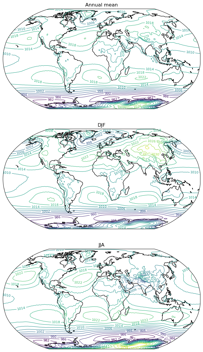
Here’s an example for the sea level pressure. I’m choosing a particular map projection here. There are lots of other choices, see the Cartopy documentation.

lon = cfsr_seas.lon
lat = cfsr_seas.lat

levels = np.arange(982., 1040., 4.)

fig, axes = plt.subplots(3, figsize=(10,15), subplot_kw={'projection': ccrs.Robinson()})

for ax in axes:
    ax.coastlines()
    
ax = axes[0]
CS = ax.contour(lon, lat, cfsr_seas.pmsl.mean(dim='season') / 100., levels=levels, linewidths=0.8, 
               transform=ccrs.PlateCarree())
ax.clabel(CS, CS.levels, inline=True, fontsize=8)
ax.set_title('Annual mean')

ax = axes[1]
CS = ax.contour(lon, lat, cfsr_seas.pmsl.sel(season='DJF') / 100., levels=levels, linewidths=0.8, 
               transform=ccrs.PlateCarree())
ax.clabel(CS, CS.levels, inline=True, fontsize=8)
ax.set_title('DJF')

ax = axes[2]
CS = ax.contour(lon,lat, cfsr_seas.pmsl.sel(season='JJA') / 100., levels=levels, linewidths=0.8, 
               transform=ccrs.PlateCarree())
ax.clabel(CS, CS.levels, inline=True, fontsize=8)
ax.set_title('JJA')

Text(0.5, 1.0, 'JJA')

../_images/8d9fcd48c9029e45c0691dae7c62b8ffd4f4356aee7383469bc7956fd2ee2daf.png

List of figures#

The following figures appear in the slide deck we saw in class, which you can find at this link (courtesy of Professor Brian Tang, University at Albany).

Our objective here is to build recipes to make all (or at least most of) these figures from the CFSR climatology.

SLP this one is already done
- annual mean
- DJF
- JJA
1000 hPa streamlines
- annual mean
- DJF
- JJA
1000 hPa zonal wind
- annual mean
- DJF
- JJA
1000 hPa meridional wind
- annual mean
- DJF
- JJA
1000 hPa temperature
- annual mean
1000 hPa zonal temperature anomaly
- DJF
- JJA
200 hPa streamlines
- annual mean
- DJF
- JJA
200 hPa zonal wind
- annual mean
- DJF
- JJA
200 hPa meridional wind
- annual mean
- DJF
- JJA
500 hPa vertical velocity (omega)
- annual mean
- DJF
- JJA
500 hPa relative humidity
- annual mean
- DJF
- JJA
850 hPa moist static energy
- annual mean
850 hPa moist static energy zonal anomaly
- DJF
- JJA
Surface enthalpy flux
- annual mean
- DJF
- JJA
Schematic: Lagrangian vs Eulerian overturning

Mass overturning circulation#

Basic ideas and theory#

An element of northward mass flux (in units of kg s\({^-1}\)) across latitude line \(\phi\) is

\[ d\psi = a \cos\phi d\lambda ~ v ~ \frac{dp}{g} \]

So the total northward mass flux across \(\phi\) above pressure level \(p\) is given by

\[\begin{align*} \psi(p) &= \int_0^{2\pi} \int_0^p a \cos\phi d\lambda ~ v ~ \frac{dp}{g} \\ &= 2\pi a \frac{\cos\phi}{g} \int_0^p [v] dp \end{align*}\]

The zonally- and time-averaged mass conservation in pressure coordinates is

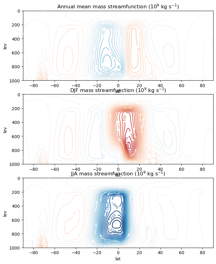
\[ \frac{1}{a \cos\phi} \frac{\partial}{\partial \phi} \left( [\overline{v}] \cos\phi \right) + \frac{\partial [\overline{\omega}]}{\partial p} = 0 \]

In other words, the vector with components \([\overline{v}], [\overline{\omega}]\) is non-divergent. So we can represent it with a scalar streamfunction \(\psi\), the mass transport streamfunction:

\[\begin{align*} 2\pi a \cos\phi [\overline{v}] &= \frac{\partial \psi}{\partial p} \\ 2\pi a^2 \cos\phi \left( [\overline{\omega}]\right) = -\frac{\partial \psi}{\partial \phi} \end{align*}\]

consistent with the definition of \(\psi\) above!

It it thus possible to compute and plot the mass streamfunction from just the zonal wind data, using

\[ \psi = \frac{2\pi a \cos\phi}{g} \int_0^p [\overline{v}] dp \]

Contours of \(\psi\) can then be interpreted as streamlines for the mean meridional circulation, that is, the zonal- and time-averaged overturning of mass in the latitude-pressure plane.

Computing the overturning streamfunction from meridonal velocities#

We’ll start by taking averages of the \(v\) data:

vbracket = cfsr_seas.v.mean(dim='lon')
vbracket

<xarray.DataArray 'v' (season: 4, lev: 40, lat: 361)>
dask.array<mean_agg-aggregate, shape=(4, 40, 361), dtype=float32, chunksize=(4, 40, 361), chunktype=numpy.ndarray>
Coordinates:
  * lat      (lat) float32 -90.0 -89.5 -89.0 -88.5 -88.0 ... 88.5 89.0 89.5 90.0
  * lev      (lev) float32 -2e-06 2e-06 10.0 20.0 ... 925.0 950.0 975.0 1e+03
  * season   (season) object 'DJF' 'JJA' 'MAM' 'SON'

It turns out that the top-most pressure level is missing in the data, e.g.:

vbracket.isel(lev=0).sel(season='DJF').values

array([nan, nan, nan, nan, nan, nan, nan, nan, nan, nan, nan, nan, nan,
       nan, nan, nan, nan, nan, nan, nan, nan, nan, nan, nan, nan, nan,
       nan, nan, nan, nan, nan, nan, nan, nan, nan, nan, nan, nan, nan,
       nan, nan, nan, nan, nan, nan, nan, nan, nan, nan, nan, nan, nan,
       nan, nan, nan, nan, nan, nan, nan, nan, nan, nan, nan, nan, nan,
       nan, nan, nan, nan, nan, nan, nan, nan, nan, nan, nan, nan, nan,
       nan, nan, nan, nan, nan, nan, nan, nan, nan, nan, nan, nan, nan,
       nan, nan, nan, nan, nan, nan, nan, nan, nan, nan, nan, nan, nan,
       nan, nan, nan, nan, nan, nan, nan, nan, nan, nan, nan, nan, nan,
       nan, nan, nan, nan, nan, nan, nan, nan, nan, nan, nan, nan, nan,
       nan, nan, nan, nan, nan, nan, nan, nan, nan, nan, nan, nan, nan,
       nan, nan, nan, nan, nan, nan, nan, nan, nan, nan, nan, nan, nan,
       nan, nan, nan, nan, nan, nan, nan, nan, nan, nan, nan, nan, nan,
       nan, nan, nan, nan, nan, nan, nan, nan, nan, nan, nan, nan, nan,
       nan, nan, nan, nan, nan, nan, nan, nan, nan, nan, nan, nan, nan,
       nan, nan, nan, nan, nan, nan, nan, nan, nan, nan, nan, nan, nan,
       nan, nan, nan, nan, nan, nan, nan, nan, nan, nan, nan, nan, nan,
       nan, nan, nan, nan, nan, nan, nan, nan, nan, nan, nan, nan, nan,
       nan, nan, nan, nan, nan, nan, nan, nan, nan, nan, nan, nan, nan,
       nan, nan, nan, nan, nan, nan, nan, nan, nan, nan, nan, nan, nan,
       nan, nan, nan, nan, nan, nan, nan, nan, nan, nan, nan, nan, nan,
       nan, nan, nan, nan, nan, nan, nan, nan, nan, nan, nan, nan, nan,
       nan, nan, nan, nan, nan, nan, nan, nan, nan, nan, nan, nan, nan,
       nan, nan, nan, nan, nan, nan, nan, nan, nan, nan, nan, nan, nan,
       nan, nan, nan, nan, nan, nan, nan, nan, nan, nan, nan, nan, nan,
       nan, nan, nan, nan, nan, nan, nan, nan, nan, nan, nan, nan, nan,
       nan, nan, nan, nan, nan, nan, nan, nan, nan, nan, nan, nan, nan,
       nan, nan, nan, nan, nan, nan, nan, nan, nan, nan], dtype=float32)

We can’t integrate over nans so we’ll replace those with zeros instead – which will make no contribution to the integral.

vbracket_zeros = vbracket.fillna(0.)

Now let’s compute the integral!

(I’m calling out to an external package to get values of the constants \(a\) (Earth radius) and \(g\) (acceleration due to gravity))

coslat = np.cos(np.deg2rad(cfsr_seas.lat))
from climlab.utils.constants import a, g

# Use units of 10^9 kg/s
psi = 2*np.pi*a*coslat/g * vbracket_zeros.cumulative_integrate(coord='lev') / 1E9 * 100
# Need to multiply by 100 because the 'lev' coordinate is in units of hPa, not Pa
psi

<xarray.DataArray (lat: 361, season: 4, lev: 40)>
dask.array<mul, shape=(361, 4, 40), dtype=float32, chunksize=(361, 4, 39), chunktype=numpy.ndarray>
Coordinates:
  * lat      (lat) float32 -90.0 -89.5 -89.0 -88.5 -88.0 ... 88.5 89.0 89.5 90.0
  * lev      (lev) float32 -2e-06 2e-06 10.0 20.0 ... 925.0 950.0 975.0 1e+03
  * season   (season) object 'DJF' 'JJA' 'MAM' 'SON'

Now we’ve got the streamfunction defined for four seasons. Time to make plots!

Plotting the mass overturning#

psi_levels = np.arange(-230, 240, 10.)

fig, axes = plt.subplots(3, figsize=(8,10))

CS = psi.mean(dim='season').plot.contour(ax=axes[0],
                                         x='lat', 
                                         yincrease=False,
                                         levels=psi_levels,
                                        )
axes[0].clabel(CS, CS.levels, inline=True, fontsize=8)
axes[0].set_title('Annual mean mass streamfunction (10$^9$ kg s$^{-1}$)')

CS = psi.sel(season='DJF').plot.contour(ax=axes[1],
                                         x='lat', 
                                         yincrease=False,
                                         levels=psi_levels,
                                        )
axes[1].clabel(CS, CS.levels, inline=True, fontsize=8)
axes[1].set_title('DJF mass streamfunction (10$^9$ kg s$^{-1}$)')

CS = psi.sel(season='JJA').plot.contour(ax=axes[2],
                                         x='lat', 
                                         yincrease=False,
                                         levels=psi_levels,
                                        )
axes[2].clabel(CS, CS.levels, inline=True, fontsize=8)
axes[2].set_title('JJA mass streamfunction (10$^9$ kg s$^{-1}$)')

Text(0.5, 1.0, 'JJA mass streamfunction (10$^9$ kg s$^{-1}$)')

../_images/61e5dd60c36aadffc0dcf49f417e7d121f5028e6ce07e9c20c58145a4e346c17.png