Introduction
We’re going to talk about three key budgets of materially conserved quantities:
Angular Momentum
Energy
Water Vapor
The general idea running through these topics is that we have a quantity that obeys some conservation principle embeded in the equations of motion, and that over a “long enough” time period that quantity must be in steady state in the atmosphere.
For any quantity in steady state, we must have a balance between local sources and sinks of that quantity and flux divergence / convergence of the same quantity.
Vertical integrals
In addition to zonal and time averages, we will sometimes employ a vertical integral (weighted by mass):
where is the surface pressure.
Angular momentum basics
The total angular momentum of the solid Earth and its fluid components is approximately conserved.
Angular momentum is exchanged between the solid Earth and the atmosphere, but on greater than annual timescales, there should be no net exchange.
Length of day
Changes in the angular momentum of the solid Earth are reflected in fluctuations of the Length of Day:
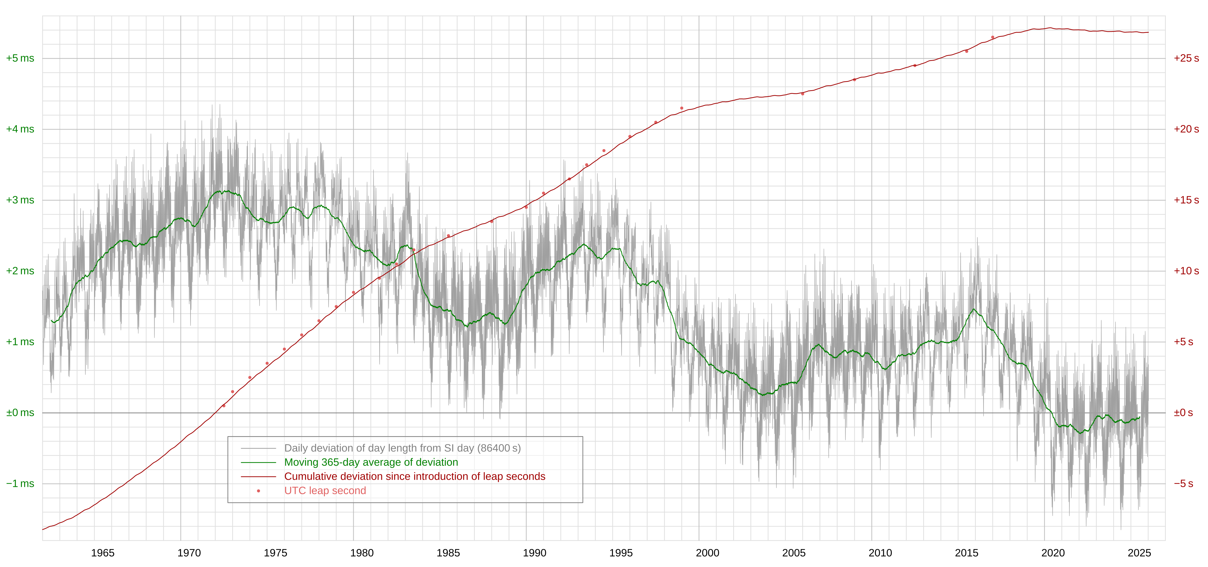
Deviation of day length from SI-based day (86’400 s) 1962–2026: daily, moving 365-day average and cumulative. For comparison, displays UTC leap seconds.
Public Domain. Source from wikimedia
There’s clearly lots of interesting low-frequency variability, but for our purposes we’ll pay most attention to the annual timescale: fluctuations of order 1 ms. It turns out that these are well-correlated with seasonal flucutations in atmospheric angular momentum.
Comparison of angular momentum to length of day variations
To show this, we’ll take a quick look at this figure reproduced from “The Atmospheric General Circulation” by Wallace et al. Wallace et al., 2023
(Top) Time series of total and relative atmospheric angular momentum AAM indicated by the red and blue curves, respectively, together with length of day LOD indicated by the black curve. The interdecadal variability in LOD attributable to motions in the Earth’s mantle has been removed and the curve has been scaled to make it comparible with the AAM curves. The scales at the left and right are different because the total AAM contains the almost constant solid body rotation component. The LOD scale in units of milliseconds is also included at the far right. (Bottom) The corresponding anomlies with respect to the seasonally varying climatological means. Courtesy of Ying Li.
Source: Wallace et al. (2023)
Definitions and notation
Let be the position vector from the axis of rotation, and let be the absolute velocity as measured in the inertial frame.
Sketch of sphere
Then we define the angular momentum
and its changes are governed by
where is the net force, and is the net torque.
Two important torques we will discuss include the frictional torque and the mountain torque.
Now define the relative velocity through
where is the Earth’s rotation vector. So the angular momentum can be written
where is a unit vector aligned with the axis of rotation. This is valid for the thin-shell approximation, where is the radius of the Earth.
The planetary component dictates the predominant direction of , so we are most interested in the component of also parallel to :
So let’s define this (scalar) quantity:
where the first term is the planetary angular momentum and the second term is the relative angular momentum .
Absolute versus relative angular momentum in seasonal extremes
The plot below is reproduced from a very nice textbook, “An Introduction to the Global Circulation of the Atmosphere” by David Randall (Colorado State University) Randall (2015).
It shows the absolute angular momentum as well as just the relative component for the seasonal extremes of January and July.
Notice that the relative component is about two orders of magnitude smaller than the absolute.

The observed absolute (left panels) and relative (right panels) atmopspheric angular momentum per unit mass, for January and July. The units are 107 m s. Source: Randall (2015)
Key features of the seasonal variations seem to be that the relative angular momentum is greater in the winter hemisphere, but also that the total integrated over the whole volume of the atmosphere seems to be larger in the N.H. winter (January).
Plotting angular momentum from ERA5 data
Let’s duplicate the plot above using one year of zonal wind () data from the ERA5.
Even though we’re just using a single year, it’s still a relatively big calculation because we start with a four dimensional dataset (lat, lon, time, and pressure levels) at hourly resolution. We’ll use some “lazy execution” tricks along the way to get our calculation done.
Lazily load the ERA5 data
See these notes for more explanation of what we’re doing here.
import numpy as np
import xarray as xr
import matplotlib.pyplot as plt
from arraylake import Client as alClient
from dask.distributed import Client as dClient
alclient = alClient()
alclient.login()repo = alclient.get_repo("earthmover-public/era5")
session = repo.readonly_session("main")
pressure_spatial = xr.open_zarr(session.store, group="pressure/spatial", chunks={})
pressure_spatial 2026-09-17T05:02:25.585628Z WARN aws_smithy_http_client::client::tls::rustls_provider::build_connector: native root CA certificate loading errors: [Error { context: "failed to read PEM from file", kind: Io { inner: Os { code: 13, kind: PermissionDenied, message: "Permission denied" }, path: "/etc/ssl/certs/sendmail.pem" } }, Error { context: "failed to read PEM from file", kind: Io { inner: Os { code: 13, kind: PermissionDenied, message: "Permission denied" }, path: "/etc/pki/tls/certs/sendmail.pem" } }]
at /home/conda/feedstock_root/build_artifacts/bld/rattler-build_icechunk_1785432413/build_env/.cargo/registry/src/index.crates.io-1949cf8c6b5b557f/aws-smithy-http-client-1.1.12/src/client/tls/rustls_provider.rs:73
Set up a dask cluster for parallelization
Tools for accelerating the data processing depend on where and how we are running the code.
We will likely get the best performance running on https://
But on a typical multicore laptop, we can still get some acceleration by invoking a local worker cluster (option 1 below).
# ## Option 1: run this on a laptop
# ##  Comment out this cell if using option 2
# dclient = dClient()
# dclient
## Option 2: If running this notebook on jupyterlab.its.albany.edu, uncomment and run this cell
## This sets up a cluster of workers to parallelize the calculations
from dask_jobqueue import SLURMCluster
cluster = SLURMCluster(cores=64, # size of a single job -- typically one node of the HPC cluster
memory="374GB", # the max memory on the 64-core burst-daes nodes, I believe
walltime="01:00:00",
queue="burst-daes",
)
cluster.adapt(minimum=1, maximum=3)
dclient = dClient(cluster)
dclientPlanetary angular momentum
First we’ll do the easy part: computing the planetary angular momentum from
We just need the planetary constants and as well as the latitude axis from our dataset:
a = 6.371E6  # the mean planetary radius in meters
sidereal_period = (23*60 + 56)*60 + 4.09053  # Earth's rotational period in seconds -- just shy of one day
Omega = 2*np.pi / sidereal_period  # Earth's angular rotation rate (radians / second)

latitude = pressure_spatial.latitude

Mplanetary = Omega * a**2 * np.cos(np.deg2rad(latitude)) / 1E7 # put in same units as Randall figure
Mplanetary.attrs['long_name'] = 'planetary angular momentum'
Mplanetary.attrs['units'] = '10^7 m^2 s^-1'
Mplanetary.plot(y='latitude');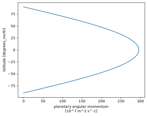
Computing relative angular momentum from zonal wind data
The formula is
This is a simple function of zonal wind and latitude (which is itself a property of the zonal wind data). Let’s go ahead and code this up as a callable Python function:
def relative_angular_momentum(u):
    '''Compute relative angular momentum in units of 10^7 m^2 s^-1'''
    value = u * a * np.cos(np.deg2rad(u.latitude)) / 1E7
    value.attrs['long_name'] = 'relative angular momentum'
    value.attrs['units'] = '10^7 m^2 s^-1'
    value.coords['geopotential_height'] = geopotential_height(value.pressure_level)
    value.geopotential_height.attrs['units'] = 'km'
    return value
We are mainly concerned here with zonal- and time averages. We will focus on the months of January and July for comparison against Randall’s figure.
For no particular reason, we will focus on the year 2021.
Side note: transforming to height coordinates
Since Randall’s figure is plotted with respect to height rather than pressure, let’s add a new coordinate dimension to our dataset that represents approximate geopotential height.
This function just computes the integrated hydrostatic balance relation for an ideal gas at a constant reference temperature (which is all we need here since it’s just for visual comparison):
def geopotential_height(p):
    '''Compute approximate geopotential height (km) from pressure based on hydrostatic balance at a reference temperature'''
    Rd = 287  # gas constant for dry air
    g = 9.8  # acceleration due to gravity
    Tref = 280.  # reference temperature in Kelvin
    ps = 1000.  # reference surface pressure in hPa
    return Rd*Tref/g * np.log(ps / p) / 1000.
We can write fully lazy code that specifies all our data transformations and reductions before actually doing any computations. Here’s an example:
#  We are NOT going to compute and plot results from this code
#  But this is to demonstrate the fully "lazy" way to set it up
u = pressure_spatial.u.sel(valid_time="2021")
Mrelative = relative_angular_momentum(u)
Mrelative_zonal = Mrelative.mean(dim='longitude')
Mrelative_monthly = Mrelative_zonal.groupby(Mrelative_zonal.valid_time.dt.month).mean(dim='valid_time')
Mrelative_monthlyWe can see that our reductions leave us with 12 individual latitude-pressure cross-sections.
Note that this is a very “cheap” operation because we haven’t actually done the computation yet!
This is an example of “lazy” execution. We’ve just set up instructions about how to calculate the result. The actual computation will only occur when it’s need (like when we try to plot a result).
It is possible to go ahead and compute the results for every month.
This commented out code would do it:
# Mrelative_monthly.compute()However, this will be very slow because of the way the data chunks are laid out.
To get decent performance, I will change the order of operations here, and focus just on the months of January and July (since those are plotted in Randall’s figure).
I’m also using the %%time magic in this cell to measure how long it takes to execute.
%%time
Mrelative_computed = {}
for name, m, interval in [("January", 1, "2021-01"), ("July", 7, "2021-07")]:
    u_zon = pressure_spatial.u.sel(valid_time=interval).mean(dim='longitude')
    u_zon_bar = u_zon.mean(dim='valid_time').compute()
    Mrelative_computed[name] = relative_angular_momentum(u_zon_bar)
CPU times: user 38.2 s, sys: 2.98 s, total: 41.1 s
Wall time: 1min 6s
And finally, let’s make the plot!
I’ll try to match the format and contour intervals of Randall’s figure.
fig, axes = plt.subplots(2,2, figsize=(16,12))

for index, mon in enumerate(['January', 'July']):
    thisMrelative = Mrelative_computed[mon]
    thisMabs = thisMrelative + Mplanetary
    CS = thisMabs.plot.contour(y='geopotential_height', levels=np.arange(10,300,20), xincrease=False, ax=axes[index,0])
    axes[index,0].clabel(CS)
    axes[index,0].set_title('Absolute angular momentum (' + mon + ' 2021)')
    CS = thisMrelative.plot.contour(y='geopotential_height', levels=np.arange(-20,32,2), xincrease=False, ax=axes[index,1])
    axes[index,1].clabel(CS)
    axes[index,1].set_title('Relative angular momentum (' + mon + ' 2021)')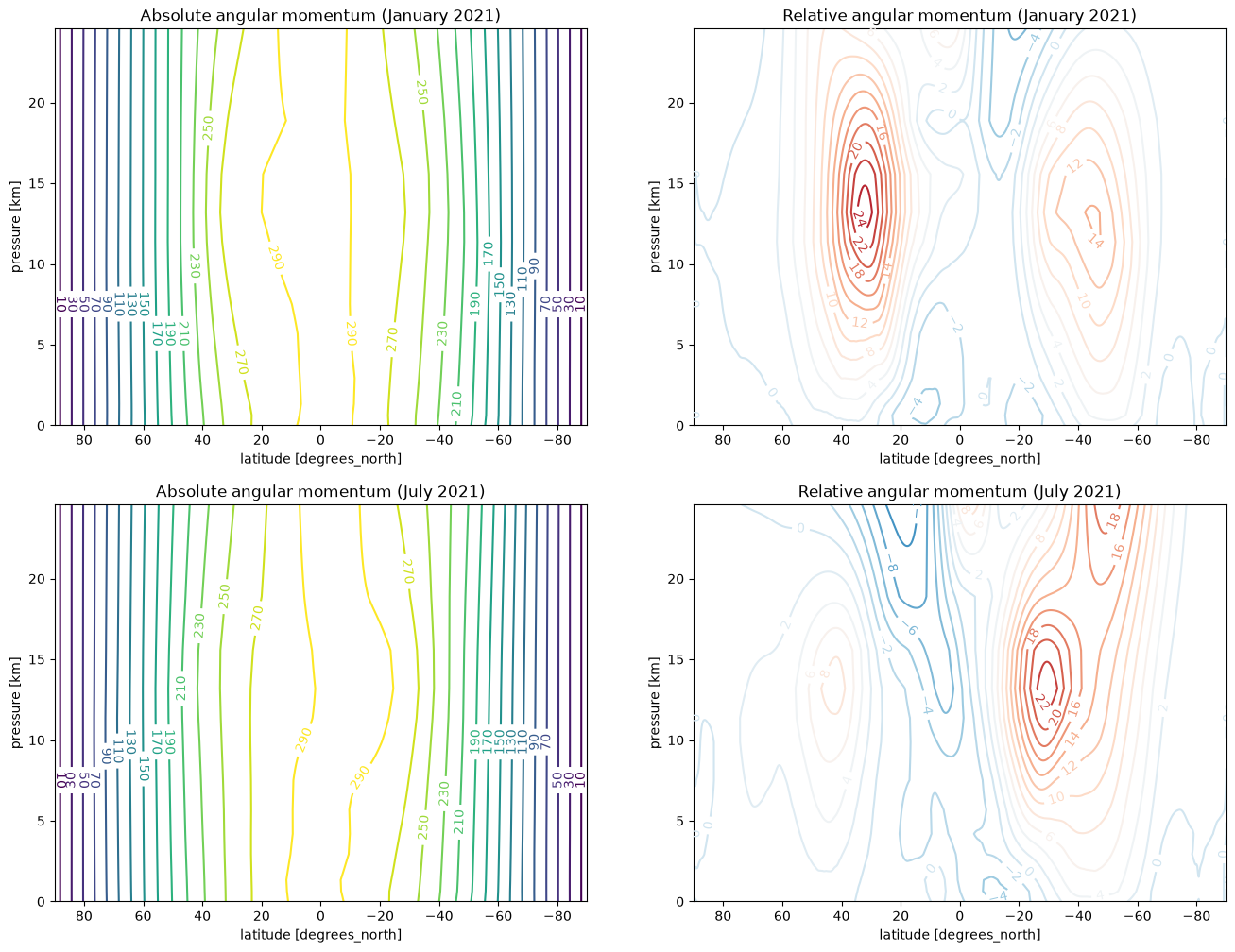
Are these figures broadly consistent with Randall’s versions? What differences do you notice?
Conservation of angular momentum
A motionless parcel moves poleward...
The total angular momentum of a parcel is conserved in the absence of torques:
or in other words, the quantity
is conserved for a moving parcel.
The fact that we live on a sphere becomes an interesting part of this problem.
Consider what happens to a parcel that starts out motionless () at the equator (). Its initial angular momentum is
Now suppose this parcel moves toward the pole. Its planetary angular momentum decreases (since is a decreasing function). This reflects the fact that the moment arm of the parcel (distance to the axis of rotation) gets smaller as the parcel moves poleward.
So to conserve total , the zonal wind must increase!
Specifically in this situation, setting and solving for gives
u_conserved = (Omega * a * np.sin(np.deg2rad(latitude))**2 / np.cos(np.deg2rad(latitude)))
u_conserved.attrs['long_name'] = 'zonal wind'
u_conserved.attrs['units'] = 'm s-1'
u_conserved.plot(xlim=(-70,70), ylim=(0,1000))
plt.grid()
plt.title('Zonal wind required for angular momentum conservation');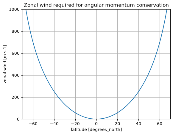
Key point here: notice that these required zonal wind values get very large (many hundreds of m/s)!
The effect of the shrinking moment arm as a parcel moves poleward seems to require much larger zonal winds that we actually observe.
Keep an eye on this as we explore the angular momentum budget of the observed atmosphere more fully.
Torques on the atmosphere
What physical processes govern changes in angular momentum in the atmosphere?
Budget equations for angular momentum
Material changes on parcels are related to partial changes through
Changes in planetary angular momentum
So we can show that changes in planetary angular momentum for a moving parcel can be written as:
This is known as the Coriolis torque.
Changes in relative angular momentum
For the relative component we can write
And we substitute in the zonal momentum equation (in “traditional” form)
to get the simplified form
Total budget
The Coriolis torque is equal and opposite in the two budgets -- it represents the exchange between planetary and relative angular momentum, and drops out of the total budget:
or, if we prefer to work in pressure coordinates,
with geopotential .
Mountain torques and frictional torques
A useful perspective here is the zonal average: let’s see what we can learn about how different processes affect the zonal mean angular momemtum.
Working in pressure coordinate and writing the equation in flux form, we take the zonal average to get:
The third term on the RHS is called the mountain torque term:
Over most of the free atmosphere, this term must be zero since the geopotential is continuous in longitude.
However, consider what happens when there are discontinuities in at fixed latitude and pressure (or equivalently, discontinuities in pressure at fixed height):
We have
This is non-zero if the pressure is different at the same height on either side of the mountain range!
Suppose we have high pressure to the west, so that . Then in this case the atmosphere pushes the mountain to the east, but the Earth exerts an equal and opposite reaction against the atmosphere to the west. The angular momentum of the atmosphere locally decreases.
Frictional torque
A reasonable starting assumption is that friction acts only at the lower boundary, and is a drag on the surface zonal wind:
with denoting the zonal wind at the surface.
Then our zonal-mean frictional torque would be
when : surface easterlies add angular momentum
when : surface westerlies remove angular momentum
The tropics act as a principle source of angular momentum and midlatitudes as the principle sink.
Areas of surface westerlies and easterlies must balance in the time mean such that angular momentum stays approximately constant
Observed torques
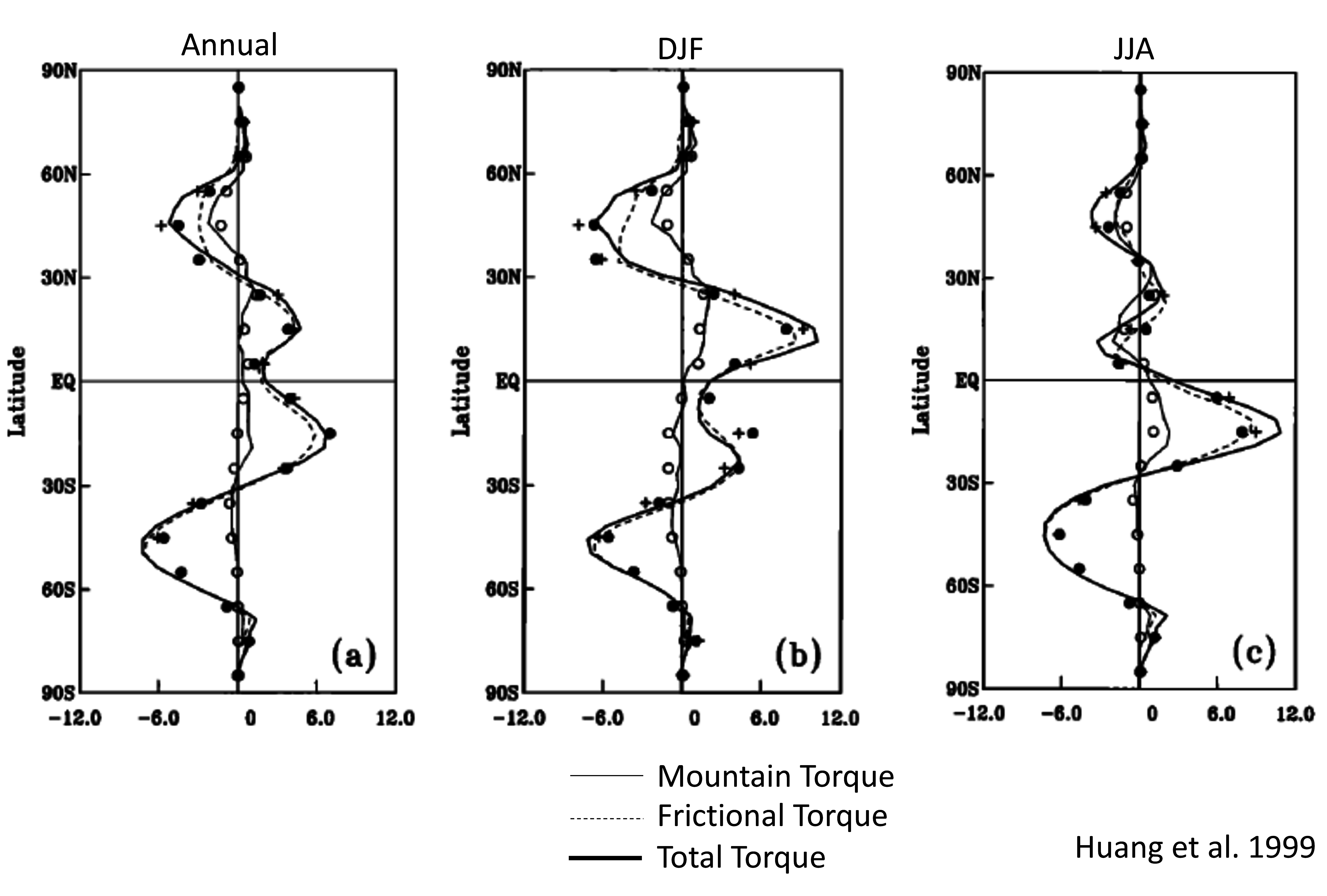
Observed zonally integrated torques on the atmosphere. Units are Hadleys per 3.8º latitude (1 Hadley = 10 kg m s. Source: Huang et al. (1999)
Some key points here:
Frictional torques generally dominate
Mountain torques are important in the N.H. midlatitudes
Winter Hadley cell is responsible for the largest angular momentum source
S.H. shows less seasonal variance (widening of frictional torque from DJF -> JJA)
Fluxes of angular momentum
The above figures of torques show that there is a net supply of angular momentum in the tropics and net sink of angular momentum* in the midlatitudes.
How does the angular momentum get redistributed with latitude?
Zonal and time averaged angular momentum budget
Let’s go back to our angular momentum budget in flux form and take the time mean:
If there an approximate balance, then the LHS of the equation goes to zero, and we must find that atmospheric transport of angular momentum supply what’s needed to balance the torques.
We now decompose the meridional flux into mean and eddy components
This equation says that the zonal, time mean meridional flux of angular momentum in comprised of
meridional flux of planetary angular momentum
meridonal flux of relative angular momentum by
mean meridional circulations
stationary eddies
transient eddies
How does this work?
The MMC transports angular momentum northward when and are positively correlated, i.e. southerlies associated with westerlies, and northerlies associated with easterlies.
Similarly for the eddy fluxes! Northward angular momentum transport results from positive correlations between and .
No net poleward transport of planetary angular momentum
We will focus mostly on the flux of relative angular momentum here. Why?
The total planetary flux, integrated with respect to mass over the depth of the atmosphere is
[Do you understand the physical argument here?]
As a consequence, it must be the fluxes of relative angular momentum that are responsible for the net meridional transport required to balance the torques.
A classic view of the vertical structure of momentum fluxes
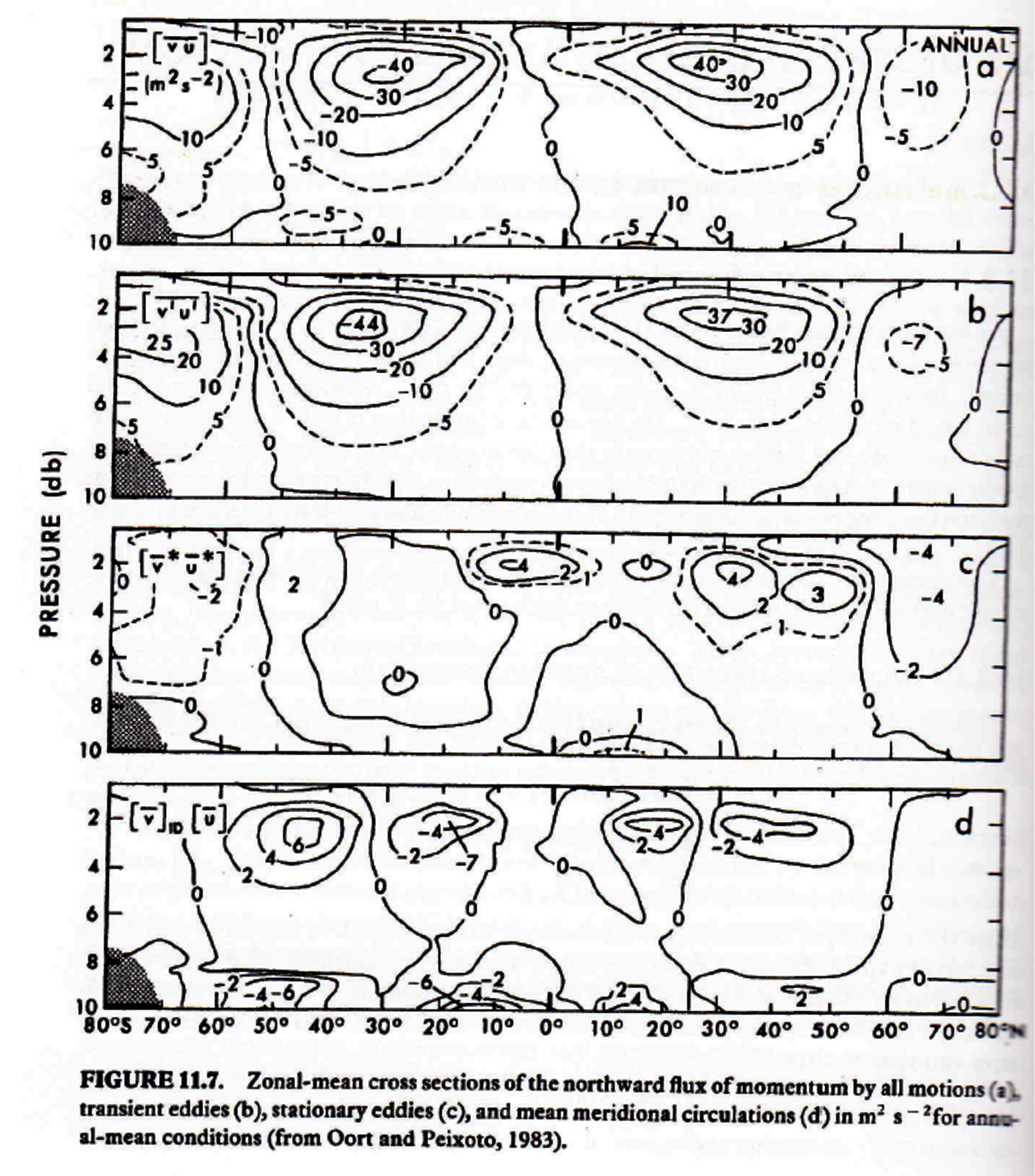
Zonal-mean cross section of the northward flux of momentum by all motions (a), transient eddies (b), stationary eddies (c), and mean meridional circulations (d) in m s for annual-mean conditions. Source: Peixoto & Oort (1992)
Let’s try to recreate this figure from the ERA5 data
We need to compute and its decomposition, so we’ll need to load data for .
v = pressure_spatial.v.sel(valid_time='2021')
v_zon = v.mean(dim='longitude')
uv = u * v
uvuv_zon = uv.mean(dim='longitude')
uv_zonuv_zon_mon = uv_zon.groupby(uv_zon.valid_time.dt.month).mean(dim='valid_time')
uv_zon_monu_zon = u.mean(dim='longitude')
u_zon_mon = u_zon.groupby(u_zon.valid_time.dt.month).mean(dim='valid_time')
v_zon = v.mean(dim='longitude')
v_zon_mon = v_zon.groupby(v_zon.valid_time.dt.month).mean(dim='valid_time')
flux_mmc = u_zon_mon * v_zon_mon
flux_mmcAnd now work on :
ustar = (u - u_zon)
vstar = (v - v_zon)
vstarustar_mon = ustar.groupby(ustar.valid_time.dt.month).mean(dim='valid_time')
vstar_mon = vstar.groupby(vstar.valid_time.dt.month).mean(dim='valid_time')
flux_stationary = (ustar_mon * vstar_mon).mean(dim='longitude')
flux_stationaryAnd finally we’ll work on .
Here we need to be careful to be consistent in the time interval we’re using to define the average and the deviation away from that average .
ubar_mon = u.groupby(u.valid_time.dt.month).mean(dim='valid_time')
vbar_mon = v.groupby(v.valid_time.dt.month).mean(dim='valid_time')

uprime_mon = u.groupby(u.valid_time.dt.month) - ubar_mon
vprime_mon = v.groupby(v.valid_time.dt.month) - vbar_mon

flux_transient = (uprime_mon * vprime_mon).groupby(u.valid_time.dt.month).mean(dim=('valid_time','longitude'))
flux_transientTime to actually compute some results!
As before, we’ll carry out the calculation for the months of January and July.
%%time
flux_total_computed = {'January': uv_zon_mon.sel(month=1).compute(),
                      'July': uv_zon_mon.sel(month=7).compute()
                     }
/network/rit/lab/snowclus/pixi/aug26/.pixi/envs/default/lib/python3.14/site-packages/distributed/client.py:3429: UserWarning: Sending large graph of size 30.32 MiB.
This may cause some slowdown.
Consider loading the data with Dask directly
or using futures or delayed objects to embed the data into the graph without repetition.
See also https://docs.dask.org/en/stable/best-practices.html#load-data-with-dask for more information.
warnings.warn(
/network/rit/lab/snowclus/pixi/aug26/.pixi/envs/default/lib/python3.14/site-packages/distributed/client.py:3429: UserWarning: Sending large graph of size 30.32 MiB.
This may cause some slowdown.
Consider loading the data with Dask directly
or using futures or delayed objects to embed the data into the graph without repetition.
See also https://docs.dask.org/en/stable/best-practices.html#load-data-with-dask for more information.
warnings.warn(
CPU times: user 1min 56s, sys: 7.7 s, total: 2min 3s
Wall time: 2min 27s
%%time
flux_mmc_computed = {'January': flux_mmc.sel(month=1).compute(),
                     'July': flux_mmc.sel(month=7).compute()
                    }
/network/rit/lab/snowclus/pixi/aug26/.pixi/envs/default/lib/python3.14/site-packages/distributed/client.py:3429: UserWarning: Sending large graph of size 40.90 MiB.
This may cause some slowdown.
Consider loading the data with Dask directly
or using futures or delayed objects to embed the data into the graph without repetition.
See also https://docs.dask.org/en/stable/best-practices.html#load-data-with-dask for more information.
warnings.warn(
/network/rit/lab/snowclus/pixi/aug26/.pixi/envs/default/lib/python3.14/site-packages/distributed/client.py:3429: UserWarning: Sending large graph of size 40.90 MiB.
This may cause some slowdown.
Consider loading the data with Dask directly
or using futures or delayed objects to embed the data into the graph without repetition.
See also https://docs.dask.org/en/stable/best-practices.html#load-data-with-dask for more information.
warnings.warn(
CPU times: user 2min 4s, sys: 7.53 s, total: 2min 11s
Wall time: 2min 39s
%%time
flux_stationary_computed = {'January': flux_stationary.sel(month=1).compute(),
                            'July': flux_stationary.sel(month=7).compute()
                           }
/network/rit/lab/snowclus/pixi/aug26/.pixi/envs/default/lib/python3.14/site-packages/distributed/client.py:3429: UserWarning: Sending large graph of size 61.17 MiB.
This may cause some slowdown.
Consider loading the data with Dask directly
or using futures or delayed objects to embed the data into the graph without repetition.
See also https://docs.dask.org/en/stable/best-practices.html#load-data-with-dask for more information.
warnings.warn(
/network/rit/lab/snowclus/pixi/aug26/.pixi/envs/default/lib/python3.14/site-packages/distributed/client.py:3429: UserWarning: Sending large graph of size 61.17 MiB.
This may cause some slowdown.
Consider loading the data with Dask directly
or using futures or delayed objects to embed the data into the graph without repetition.
See also https://docs.dask.org/en/stable/best-practices.html#load-data-with-dask for more information.
warnings.warn(
CPU times: user 3min 11s, sys: 11.5 s, total: 3min 23s
Wall time: 4min 49s
%%time
flux_transient_computed = {'January': flux_transient.sel(month=1).compute(),
                           'July': flux_transient.sel(month=7).compute()
                          }
/network/rit/lab/snowclus/pixi/aug26/.pixi/envs/default/lib/python3.14/site-packages/distributed/client.py:3429: UserWarning: Sending large graph of size 63.57 MiB.
This may cause some slowdown.
Consider loading the data with Dask directly
or using futures or delayed objects to embed the data into the graph without repetition.
See also https://docs.dask.org/en/stable/best-practices.html#load-data-with-dask for more information.
warnings.warn(
/network/rit/lab/snowclus/pixi/aug26/.pixi/envs/default/lib/python3.14/site-packages/distributed/client.py:3429: UserWarning: Sending large graph of size 63.57 MiB.
This may cause some slowdown.
Consider loading the data with Dask directly
or using futures or delayed objects to embed the data into the graph without repetition.
See also https://docs.dask.org/en/stable/best-practices.html#load-data-with-dask for more information.
warnings.warn(
CPU times: user 3min 32s, sys: 12.9 s, total: 3min 45s
Wall time: 6min 4s
Now it’s time to make some plots
Let’s make a plot like the one above from Peixoto and Oort showing the vertical cross-section of the fluxes and their decomposition
month = 'January'
levs = np.arange(-80,85,10)

fig, axes = plt.subplots(4,1, figsize=(8,12))

for num, flux in enumerate([flux_total_computed,
                             flux_mmc_computed,
                             flux_stationary_computed,
                             flux_transient_computed]
                           ):
    CS = flux[month].plot.contour(ax=axes[num],
                                  yincrease=False,
                                  levels=levs,
                                 )
    axes[num].clabel(CS)

axes[0].set_title(r'Total momentum flux $[\overline{uv}]$ (January)')
axes[1].set_title(r'Momentum flux by MMC $[\overline{u}][\overline{v}]$ (January)')
axes[2].set_title(r'Momentum flux by stationary eddies $[\overline{u}^* \overline{v}^*]$ (January)')
axes[3].set_title(r'Momentum flux by transient eddies $[\overline{u^\prime v^\prime}]$ (January)');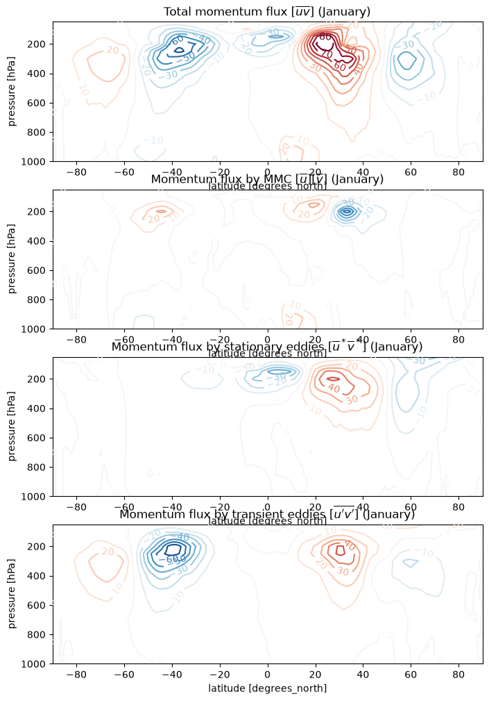
A few things to note here:
The transient eddy term is large at upper levels
The stationary eddy term is also large in the Northerm Hemisphere winter (stationary waves)
MMC term is smaller but carries the signature of the overturning circulation
What does this look like in the opposite season?
month = 'July'
levs = np.arange(-80,85,10)

fig, axes = plt.subplots(4,1, figsize=(8,12))

for num, flux in enumerate([flux_total_computed,
                             flux_mmc_computed,
                             flux_stationary_computed,
                             flux_transient_computed]
                           ):
    CS = flux[month].plot.contour(ax=axes[num],
                                  yincrease=False,
                                  levels=levs,
                                 )
    axes[num].clabel(CS)

axes[0].set_title(r'Total momentum flux $[\overline{uv}]$ (July)')
axes[1].set_title(r'Momentum flux by MMC $[\overline{u}][\overline{v}]$ (July)')
axes[2].set_title(r'Momentum flux by stationary eddies $[\overline{u}^* \overline{v}^*]$ (July)')
axes[3].set_title(r'Momentum flux by transient eddies $[\overline{u^\prime v^\prime}]$ (July)');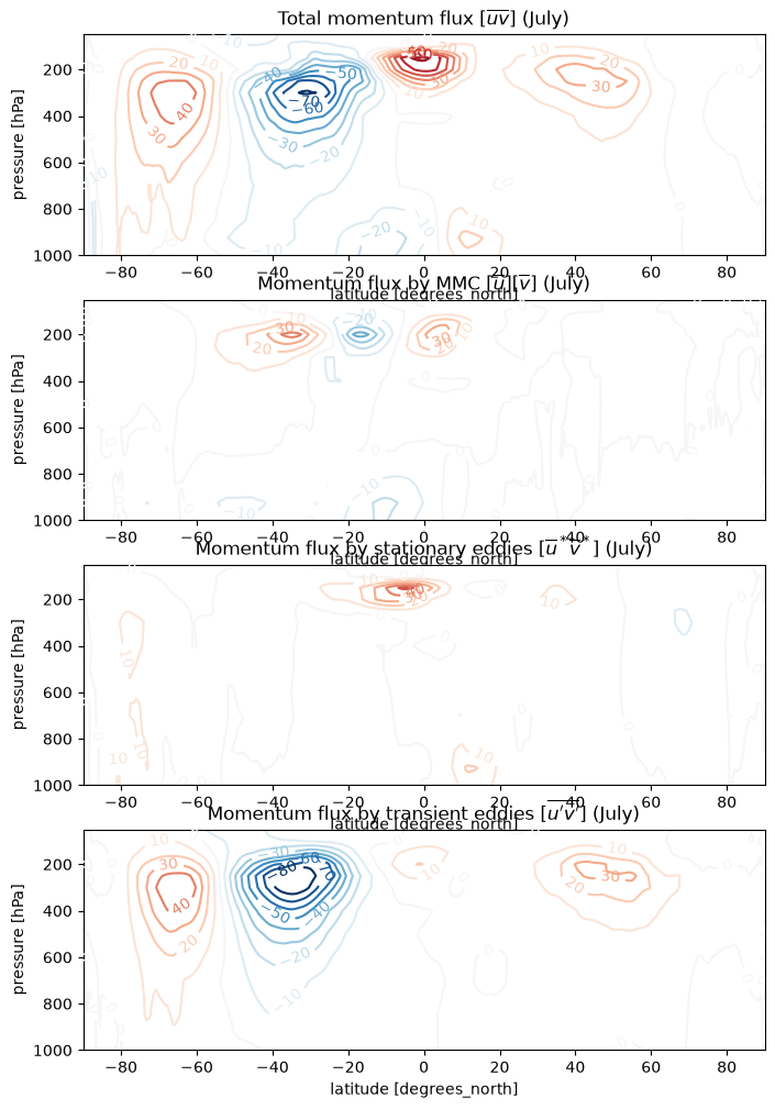
The transient eddy term dominates the Southern Hemisphere winter. As usual, the stationary eddy term is small in this season (winter in the South, summer in the North)
A vertically integrated view
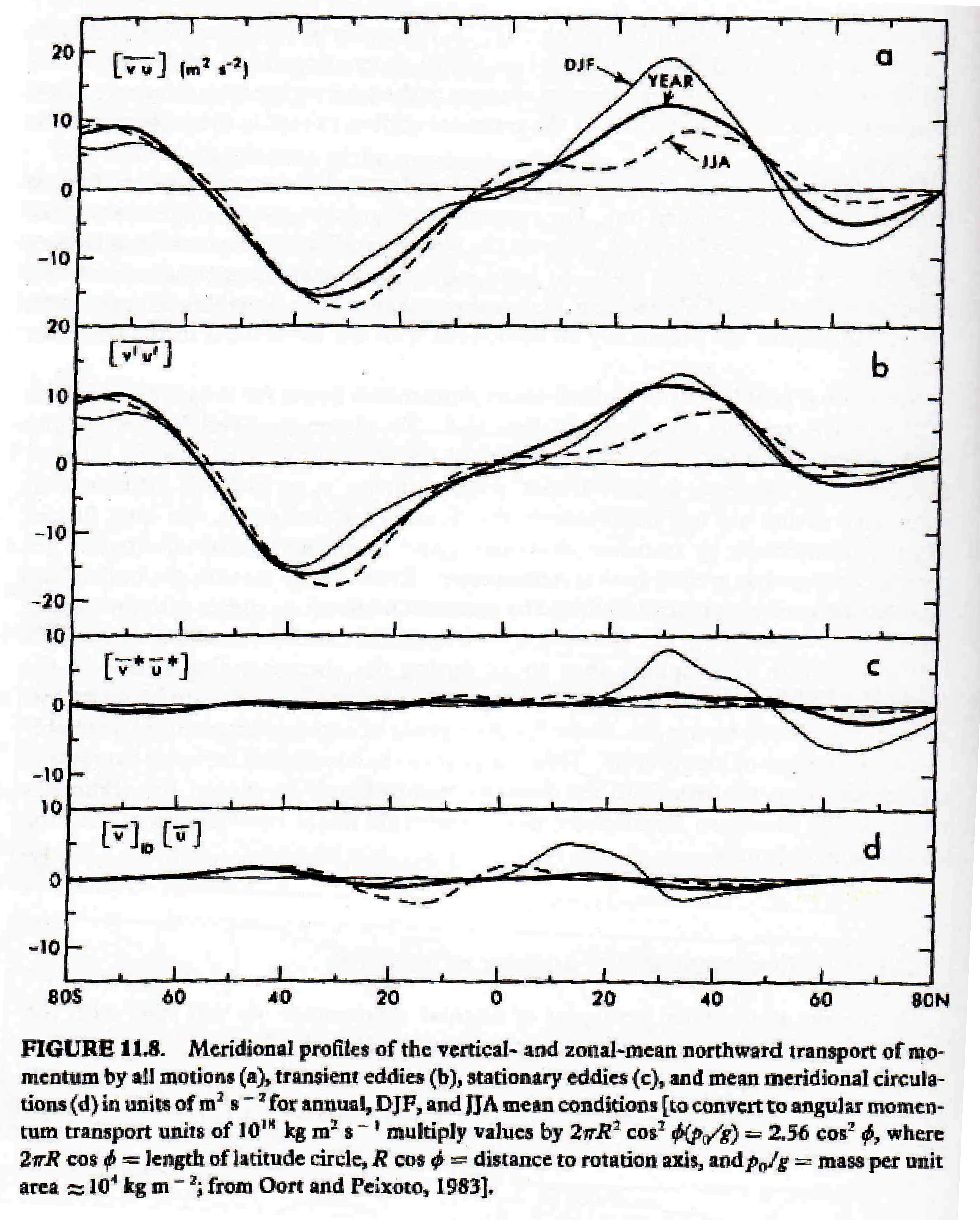
Meridional profiles of the vertical- and zonal-mean northward transport of momentum by all motions (a), transient eddies (b), stationary eddies (c), and mean meridional circulations (d) in units of m s for annual, DJF, and JJA mean conditions. Source: Peixoto & Oort (1992)
Seasonal cycle more apparent in N.H.
Transient eddy component still dominates
MMC component more important at solstices than suggested by the annual mean
S.H. slightly greater peak flux of angular momentum compared to N.H. (compensation by the ocean?)
Streamlines of angular momentum flux
In the long term mean, we suppose there’s a steady state at each latitude
so the steady-state budget looks like
Now for notational convenience, let’s wrap all our torques together like this:
and subtract out the planetary angular momentum flux since it can’t contribute to net poleward transport of absolute angular momentum.
The budget becomes
Let’s now define an angular momentum streamfunction as follows:
The streamfunction is a function in the plane whose contours give the direction of the angular momentum transport.
A plot of the streamlines
This gives a visual sense of the direction of angular momentum transport by various components of the flow:
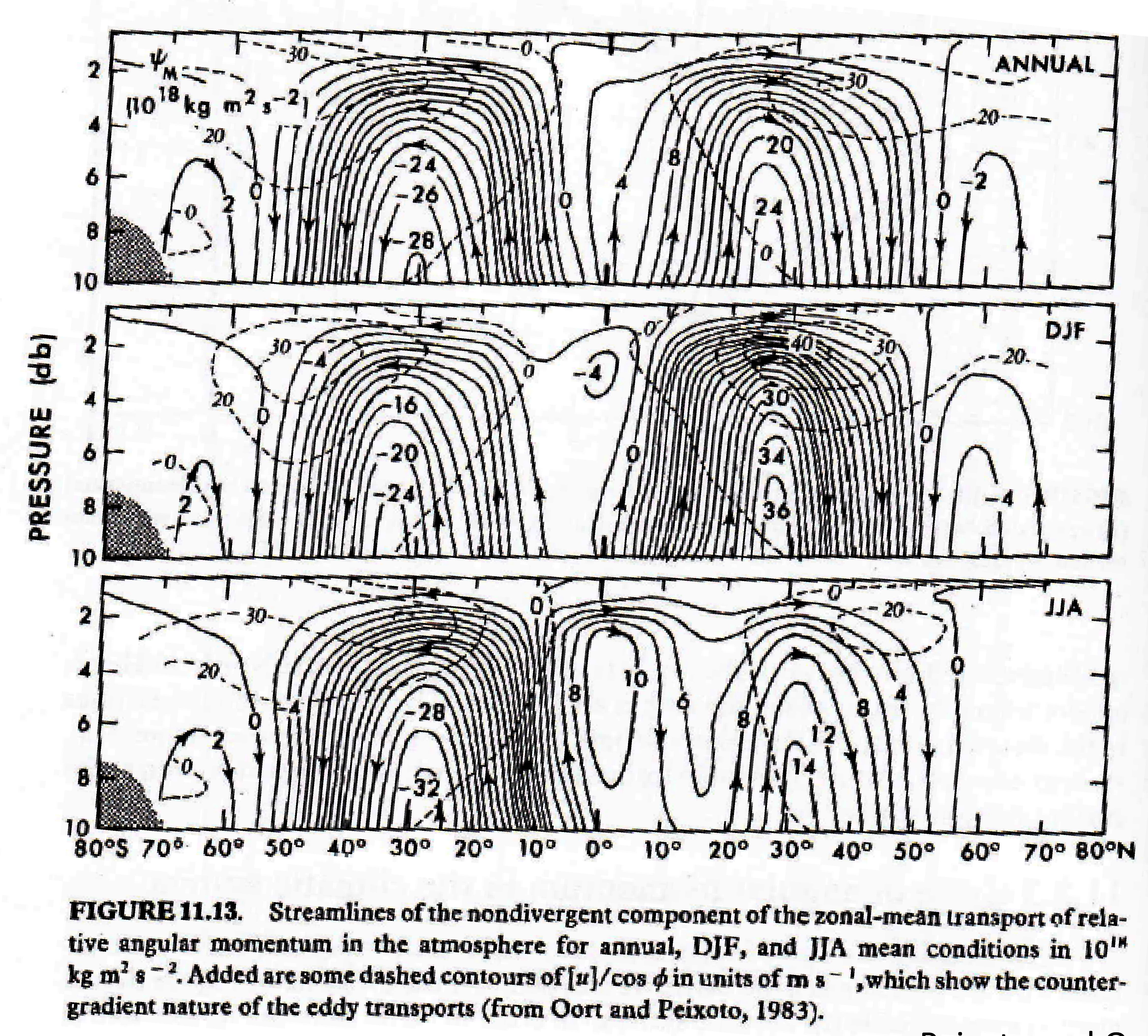
Streamlines of the nondivergent component of the zonal-mean transport of relative angular momentum in the atmosphere. Source: Peixoto & Oort (1992)
Some things to note here:
We have a near-surface source of angular momentum in the tropics (frictional torque associated with easterly trade winds)
There is upward tranpsort of angular momentum by the mean meridional circulation in the tropics / subtropics
Horizontal (poleward) transport of angular momentum in upper tropopsphere associated with eddies
Downward transport in the midlatitudes
A sink in westerly angular momentum in midlatitudes (frictional torque associated with surface westerlies)
Seasonally, the main source of angular momentum is in the tropics / subtropics of the winter hemisphere where the easterly trades are strongest.
Clean up our computational environment
When we are done with the number crunching, we should close the cluster and release those resources back to the next user.
cluster.close()- Wallace, J. M., Battisti, D. S., Thompson, D. W. J., & Hartmann, D. L. (2023). The Atmospheric General Circulation. Cambridge University Press.
- Randall, D. (2015). An Introduction to the Global Circulation of the Atmosphere. Princeton University Press.
- Huang, H.-P., Sardeshmuhk, P. D., & Weickmann, K. M. (1999). The balance of global angular momentum in a long-term atmospheric data set. J. Geophys. Res. Atmos., 104(D2), 2031–2040. 10.1029/1998JD200068
- Peixoto, J. P., & Oort, A. H. (1992). Physics of Climate. Springer-Verlag.