Motivation
We saw at the end of the last set of notes that both eddy momentum fluxes and eddy heat (buoyancy) fluxes are both involved in determing the zonal-mean flow:
Let’s consider the effects of an eddy heat flux on a frictionless, adiabatic system ().
At steady state, the thermodynamic equation tells us that we must have an Eulerian mean overturning circulation with vertical component
which in turn, by mass conservation, requires a horizontal component of the overturning .
But enters into the momentum equation through the Coriolis force.
So, eddy heat fluxes must accelerate the zonal mean zonal wind through Coriolis forces associated with the overturning circulation. Eddy heat fluxes appear in the zonal mean momentum equation disguised as Coriolis force.
Are you confused yet?
Maybe there’s a better way to express the combined effect of eddy heat and momentum fluxes that clarify under what conditions the eddies can accelerate the mean zonal flow .
[Related, we’ve also seen that the Lorenz cycle reveals substantial conversion from eddy kinetic energy to kinetic energy of the mean flow]
Along the way, we may also find a better way to think about the overturning circulation in a flow dominated by eddies.
The Transformed Eulerian Mean (TEM) or “Residual Circulation”
The residual overturning required by diabatic heating
Define a “residual” vertical motion as the direct response to diabatic heating, accounting for the large cancellation between eddy heat flux convergence and adiabatic ascent:
where we have just wrapped the eddy heat flux term into :
So far, just clever notation.
Now, let’s define the horizonal component of the residual overturning to obey mass continuity:
So between and the Eulerian mean must be
Together describe a residual overturning circulation specifically required by the diabatic heating!
Acceleration of the zonal mean wind
Now let’s use this to rewrite the momentum equation in terms of the Coriolis force due to :
or, rewriting with only eddy forcing terms on the RHS:
This is actually a deep result. is determined entirely by the zonal diabatic heating, regardless of what the eddies are doing. Our transformed momentum equation tells that there’s a very specific combination of eddy heat and momemtum fluxes that accelerate the zonal mean wind.
The transformed equation no longer has any “hidden” eddy effects -- it expresses more completely how the eddies drive the mean flow.
The Eliassen-Palm flux vector
It’s useful and traditional to define a vector (in the latitude-height plane) whose divergence appears on the RHS of the momentum equation. That is, we want to write the Transformed Eulerian Mean system like this:
From the transformed momentum equation above, we can see that
the vertical component of must be propotional to eddy heat flux
the horizontal component of must be proportional to eddy momentum flux (but in reverse direction)
More precisely, we can define for this system like this:
The vector is called the Eliassen-Palm flux, after a pioneering paper by Eliassen & Palm (1961).
A potential vorticity perspective
The idea
We’ve been talking about combining momentum and thermodynamic constraints together into a single quantity . That may sound familiar.
Recall that under the Quasi-Geostrophic approximation, we boil down all the dynamics into a single prognostic scalar, the quasi-geostrophic potential vorticity (QGPV). We might therefore expect a deep relationship between PV dynamics and the Eliassen-Palm flux .
And there is!
Zonal average QGPV equation
Let’s write
[Need to fill in details here]
The key result
The divergence of the EP flux (which is a specific combination of eddy heat and momentum fluxes) is equivalent to a northward eddy flux of QGPV!
So another form of the TEM equations is (under the quasi-geostrophic approximation):
A perspective on the steady, balanced circulation
For a balanced time-mean flow, our TEM equations thus say
Now consider the fact that the diabatic heating tends to decrease from equator to pole. So might be upward near the equator and downward near the pole.
We infer from this that must be poleward aloft (to conserve mass) -- i.e. . The residual circulation should look something like a big equator-to-pole scale Hadley cell!
But this poleward residual circulation applies an eastward Coriolis force on the zonal wind. To have a steady balance, the eddies must be arranged to produce an equal and opposite westward force.
We can infer from this that the eddies must be fluxing QGPV equatorward, i.e.
Since the planetary PV increases toward the poles, the eddies are thus flux PV down the mean gradient. Unlike for momentum, the eddies behave diffusively in the PV framework -- acting to transport PV from the high reservoir near the poles to the low reservoir near the equator.
TEM equations for the atmosphere
The theory and diagnostic method are laid out in a well-known paper by Edmon Jr. et al. (1980).
The EP flux vector components for the atmosphere
The appropriate definitions for the components of are
where we now use pressure coordinates, measure buoyancy using potential temperature , and we have defined a stratification parameter
Note that for statically stable conditions since increases upward.
Complete set of TEM equations for the atmosphere
TEM equations for the atmosphere on a sphere look like
The residual mean for the atmosphere
Definitions for and consistent with the above equations are
An angular momentum equation
The Eulerian mean angular momentum is
so the transformed zonal momentum equation can also be expressed in terms of angular momentum as
to quasi-geostrophic order.
This form shows that the divergence of the EP flux is a direct eddy forcing on the zonal mean angular momentum -- a torque on the atmosphere!
Plotting the Eliassen-Palm cross-section from reanalysis data
The classic figure
We are going to make an updated version of this famous figure showing and its divergence:
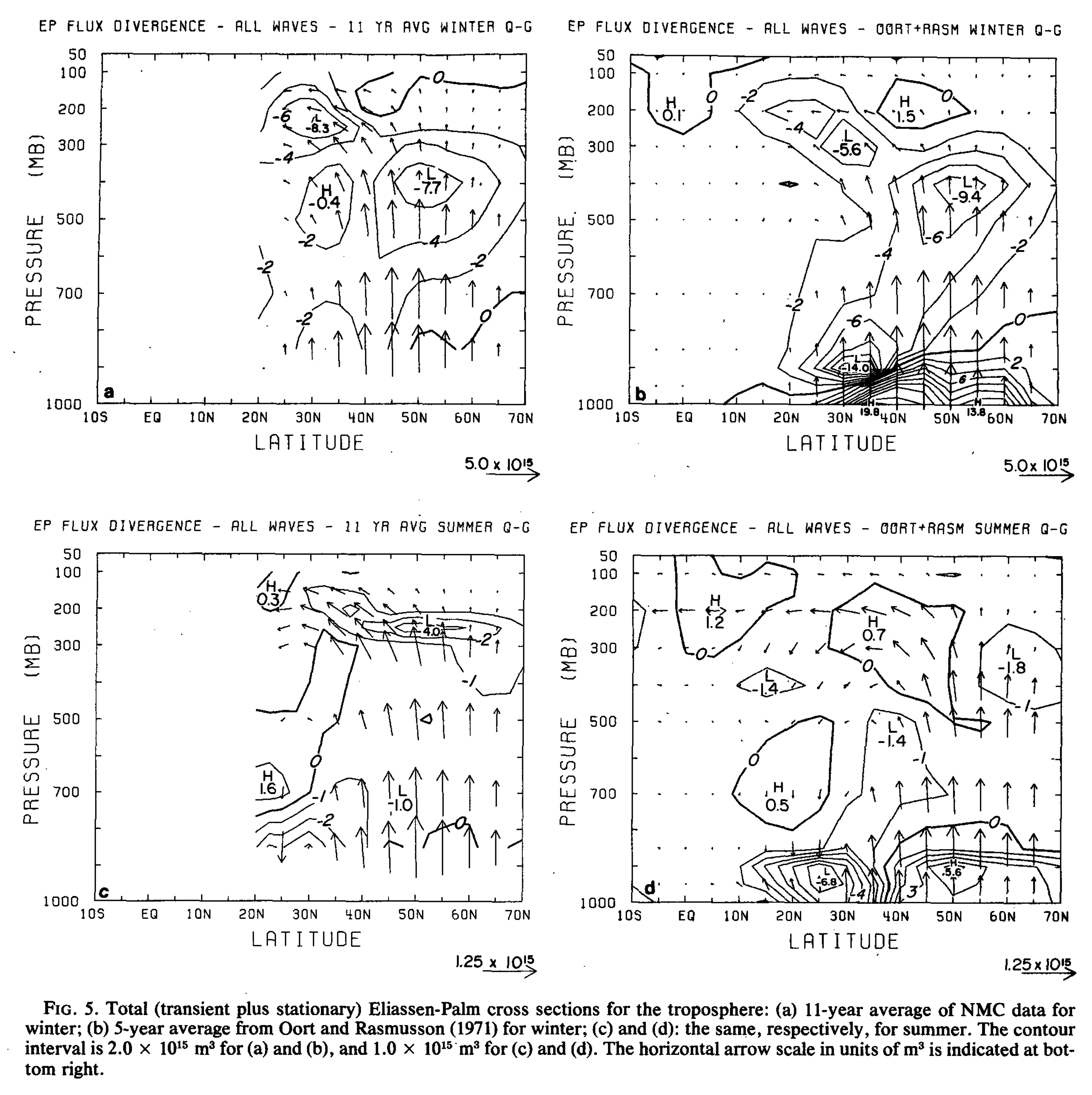
Source: Edmon Jr. et al. (1980) (Their Figure 5).
Load the CFSR data and get to work
import xarray as xr
import numpy as np
import matplotlib.pyplot as plt
from dask_jobqueue import SLURMCluster
from dask.distributed import Client
cluster = SLURMCluster(processes=4, #By default Dask will run one Python process per job.
# However, you can optionally choose to cut up that job into multiple processes
cores=80, # size of a single job -- typically one node of the HPC cluster
memory="376.2GB", # the max memory on the 80-core batch nodes, I believe
walltime="04:00:00",
queue="batch",
)
cluster.scale(1)
client = Client(cluster)
clientyears = range(2008,2018) # Ten years of data 2008 through 2017
variables = ['u', 'v', 't']
path_to_cfsr_data = '/network/daes/cfsr/data/'
ending = '.0p5.anl.nc'
files = []
for year in years:
for var in variables:
filepath = path_to_cfsr_data + str(year) + '/' + var + '.' + str(year) + ending
files.append(filepath)cfsr_6hourly = xr.open_mfdataset(files, chunks={'time':10, 'lev': 32})
cfsr_6hourlyv = cfsr_6hourly.v
u = cfsr_6hourly.u
T = cfsr_6hourly.tfrom climlab.utils.constants import Rd, cp, a, g
sidereal_period = (23*60 + 56)*60 + 4.09053 # Earth's rotational period in seconds -- just shy of one day
Omega = 2*np.pi / sidereal_period # Earth's angular rotation rate (radians / second)p = cfsr_6hourly.lev * 100. # in units of Pa
phi = np.deg2rad(cfsr_6hourly.lat) # in units of radians
from numpy import cos, sin
f = 2*Omega*sin(phi) # everyone's favorite Coriolis parameterpref = 1000. # reference pressure in hPa
kappa = Rd/cp
theta = T * (pref/cfsr_6hourly.lev)**kappadef bracket(data):
return data.mean(dim='lon', skipna=True)
def star(data):
return data - bracket(data)
def bar(data, interval=cfsr_6hourly.time.dt.season):
return data.groupby(interval).mean(skipna=True)
def prime(data, interval=cfsr_6hourly.time.dt.season):
return data.groupby(interval) - bar(data, interval=interval)heatflux = bar(bracket(star(v) * star(theta)))heatfluxCompute for solstice seasons:
heatflux_computed = {}
for season in ['DJF', 'JJA']:
    heatflux_computed[season] = heatflux.sel(season=season).load()
levels = np.arange(-400, 401, 5)
fig, axes = plt.subplots(2,1,figsize=(8,12))
for ind, season in enumerate(['DJF', 'JJA']):
ax = axes[ind]
thisflux = heatflux_computed[season]
CS = thisflux.plot.contour(ax=ax,
yincrease=False,
levels=levels,
colors='royalblue',
)
ax.clabel(CS, CS.levels, inline=True, fontsize=8)
ax.set_title('Eddy heat flux (K m/s), 2008-2017 {}'.format(season))
ax.grid()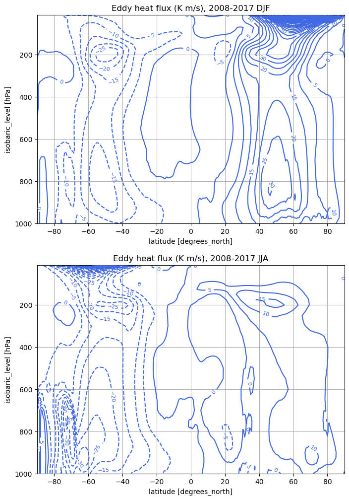
momentumflux = bar(bracket(star(v) * star(u)))momentumflux_computed = {}
for season in ['DJF', 'JJA']:
momentumflux_computed[season] = momentumflux.sel(season=season).load()levels = np.arange(-100, 101, 10)
fig, axes = plt.subplots(2,1,figsize=(8,12))
for ind, season in enumerate(['DJF', 'JJA']):
ax = axes[ind]
thisflux = momentumflux_computed[season]
CS = thisflux.plot.contour(ax=ax,
yincrease=False,
levels=levels,
colors='royalblue',
)
ax.clabel(CS, CS.levels, inline=True, fontsize=8)
ax.set_title('Eddy momentum flux (m2/s2), 1988-2017 {}'.format(season))
ax.grid()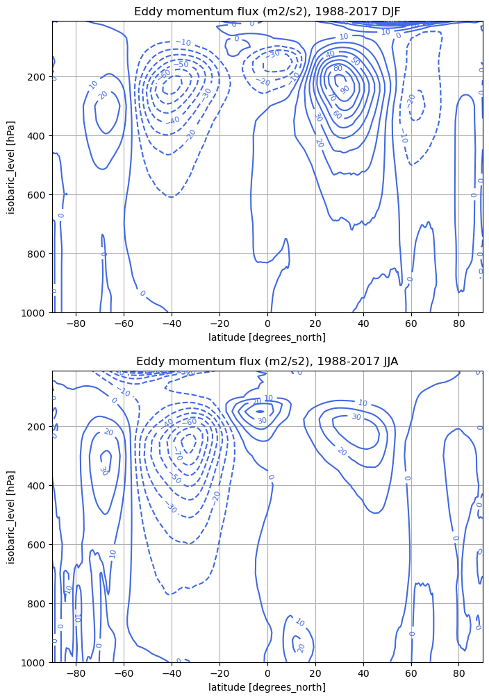
theta_zon = bar(bracket(theta))
sigma = theta_zon.differentiate(coord='lev') / 100.  # convert from K / hPa to K / Pa
sigma_computed = {}
for season in ['DJF', 'JJA']:
sigma_computed[season] = sigma.sel(season=season).load()levels = np.arange(-0.1, 0., 0.0005)
fig, axes = plt.subplots(2,1,figsize=(8,12))
for ind, season in enumerate(['DJF', 'JJA']):
ax = axes[ind]
thissigma = sigma_computed[season]
CS = thissigma.plot.contour(ax=ax,
yincrease=False,
levels=levels,
colors='royalblue',
)
ax.clabel(CS, CS.levels, inline=True, fontsize=8)
ax.set_title('Stratification parameter (K / Pa), 2008-2017 {}'.format(season))
ax.grid()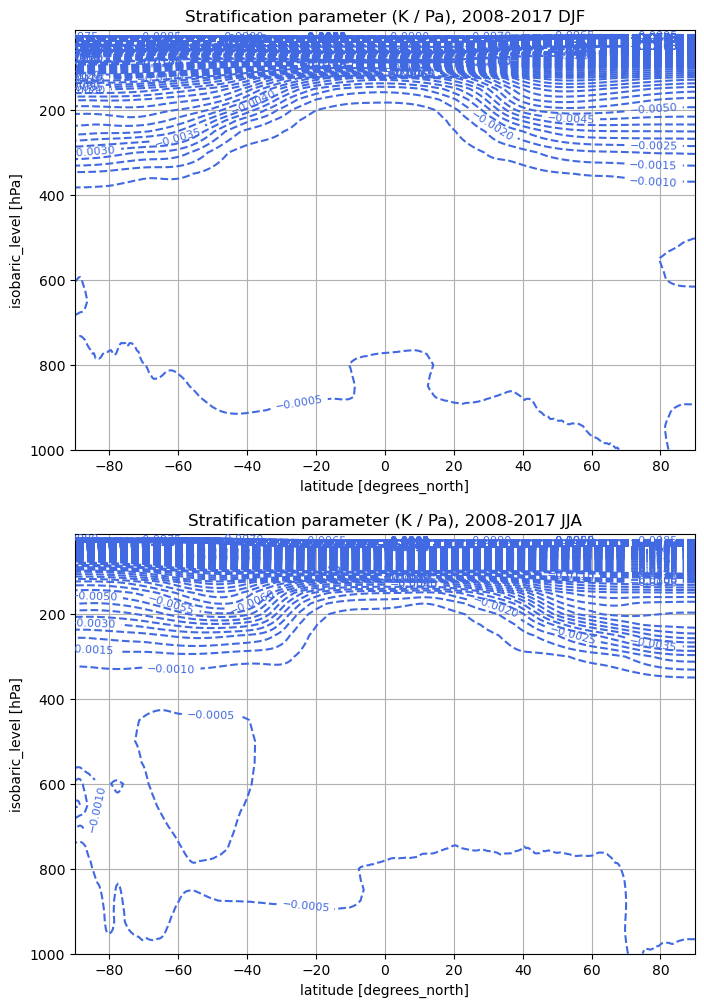
The rescaled “hat” components
Define the quantity as
where
so that is the divergence of weighted by the mass of the annulus .
Plotting the EP flux diagram
We will plot contours of to best represent the eddy forcing of the mean flow. Note that has dimensions of length cubed.
Similarly, we will represent by plotting arrows whose horizontal and vertical components are respectively proportional to and . However we re-scale the vertical component by a factor related to the aspect ratio of the plot: vertical distance per Pa / horizontal distance per radian.
This allows for a more natural visual interpretation of the plot, since arrow lengths in the horizontal and vertical now correspond directly to their contribution to the divergence.
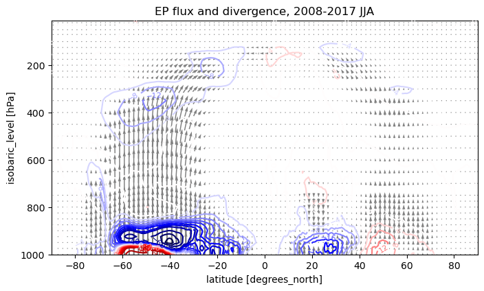
The resulting graph is precisely the Eliassen-Palm cross-section defined by Edmon Jr. et al. (1980).
def compute_ep_flux(heatflux, momentumflux, sigma, aspect=0.1):
    '''aspect is vertical distance per hPa / horizontal distance per degree (in figure units)'''

    # Calculate the physical div F (not the hat version that is used for plotting, see Edmon et al.)
    F_phi = -a * cos(phi) * momentumflux  # in units of m^3/s^2
    F_p = f * a * cos(phi) * heatflux / sigma  # in units of Pa m^2/s^2
    # The rescaled "hat" components
    Fhat_phi = (2*np.pi*a/g) * cos(phi) * F_phi  # in units of m^3
    Fhat_p = (2*np.pi*a**2/g) * cos(phi) * F_p   # in units of Pa m^3
    # Compute divergence
    Delta_phi = Fhat_phi.differentiate(coord='lat')  # In m^3 / degree
    Delta_phi *= 180./np.pi  # Now in m^3 / radian = m^3
    Delta_p = Fhat_p.differentiate(coord='lev')  # Now in Pa m^3 / hPa
    Delta_p /= 100.  # In Pa m^3 / Pa = m^3
    Delta = Delta_phi + Delta_p  # in units of m^3

    aspect = 0.1 # vertical distance per hPa / horizontal distance per degree (in figure units)
    A = aspect / 100. * np.pi / 180.  # vertical distance per Pa / horizontal distance per radian

    # multiply the F_p component by A so that the arrows are properly scaled.
    # The factor -1 is necessary to correct a sign issue with the quiver plot
    # Presumably because the pressure axis is increasing downward
    Fhat_scaled = xr.Dataset({"Fhat_phi": Fhat_phi, "Fhat_p": Fhat_p * A * -1})

    # If we plot the data as-is, there will be far too many arrows because of the high spatial resolution of the data.
    # We will down-sample in the latitude dimension before plotting the arrows.
    coarseFhat = Fhat_scaled.coarsen(lat=4, boundary="pad").mean()

    return Delta, Delta_phi, Delta_p, coarseFhat
Delta = {}
Delta_phi = {}
Delta_p = {}
coarseFhat = {}
for season in ['DJF', 'JJA']:
Delta[season], Delta_phi[season], Delta_p[season], coarseFhat[season] = \
compute_ep_flux(heatflux_computed[season],
momentumflux_computed[season],
sigma_computed[season])def epfluxplot(Delta, Fhat, label='DJF', aspect=0.1):
levels = [-100, -80, -60, -40,
-35, -30, -25, -20, -16, -12, -8, -4, 0,
4, 8, 12, 16, 20, 25, 30, 35, 40, 60, 80, 100,
]
fig, ax = plt.subplots(figsize=(8,6))
ax.set_aspect(aspect)
CS = (Delta/1E15).plot.contour(ax=ax,
x='lat',
yincrease=False,
levels=levels,
cmap='seismic',
)
ax.clabel(CS, CS.levels, inline=True, fontsize=8)
Fhat.plot.quiver(ax=ax, x="lat", y="lev",
u="Fhat_phi", v="Fhat_p",
color='gray')
ax.set_title('EP flux and divergence, 2008-2017 {}'.format(label))
return fig, axfor season in ['DJF', 'JJA']:
fig, ax = epfluxplot(Delta[season], coarseFhat[season], label=season)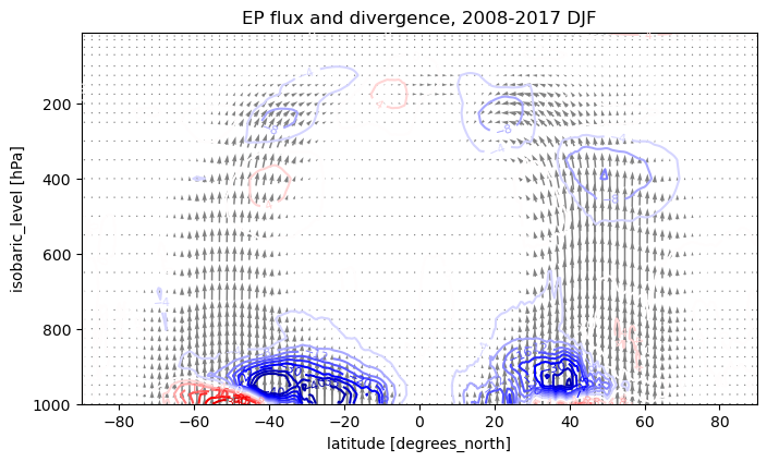
Interpreting the EP flux diagram
In the winter hemisphere, the flux is convergent throughout much of the midlatitude troposphere, indicating that the eddy fluxes are acting to decelerate the zonal wind.
This effect is concentrated into three lobes, respectively centered at roughly (35º, 850 hPa), (50º, 500 hPa) and (20º, 250 hPa) in both winter hemispheres.
Strongest divergences and convergences occur near the lower boundary.
Strongly divergent flux in the lowest levels throughout much of the mid-latitudes.
Consistent with quasi-geostrophic theory in the presence of a meridional temperature gradient, which forces to zero at the boundary but strongly divergent immediately above the boundary.
The net effect of the eddy fluxes (in the winter season at least) is a
deceleration of the zonal wind aloft, and
acceleration near the surface.
In other words, the eddies are acting to neutralize the vertical shear, or through the thermal wind balance, to neutralize the meridional temperature gradient.
The divergence near the boundary does not show a strong seasonal variation. Away from the boundary, the fluxes and their divergences become significantly weaker in the summer season. This is consistent with greater eddy activity in the winter season, especially in the NH.
One of the big advantages of presenting the eddy flux data in the form of EP cross-sections is that it gives us an immediate visual indication of the relative importance of eddy heat and momentum fluxes to the eddy PV flux.
Arrows in our EP diagrams are nearly vertical throughout most of the troposphere, indicating the dominance of the eddy heat fluxes.
The arrows have a horizontal component in the subtropical upper troposphere.
This is the region where the momentum flux is strongly divergent, as we saw above.
Our EP flux diagram gives a more complete picture of the eddy forcing of the mean flow than the original Eliassen-Palm cross-sections presented by Edmon Jr. et al. (1980), due to the global span and higher resolution of our data.
Concluding remarks about the Eliassen-Palm flux plots
Quoting from the summary from Edmon Jr. et al. (1980):
EP cross sections and the transformed mean-flow equations furnish a powerful and practical way of viewing the dynamics of eddies on a zonal wind, whether in the troposphere or in the middle atmosphere, and whether or not the eddies are well described by linear wave theory... The information displayed on an EP cross section comes as close to the heart of the eddy, mean flow interaction problem as seems likely to be possible for any Eulerian diagnostic...
They furthermore throw out some ideas for future work:
For the troposphere it would be of great interest to see the EP cross sections for different zonal wave-numbers... Individual days would be of interest as well as seasonal averages. If such cross sections could be obtained despite the formidable data-quality problems, they would give a revealing view of the horizontal, vertical and temporal structure of the interactions among different kinds of eddy and the zonal-mean state.
Now that reanalysis datasets have largely solved the “formidable data-quality problems”, it would be great fun to revisit some of these problems.
The residual mean overturning
The idea
We’ve defined a residual meridonal velocity
that is “corrected” by the eddy heat fluxes that we already computed.
What is the mass-conserving overturning associated with this ? It should get us a little closer to a Lagrangian perspective, that is, what is the typical trajectory experienced by a parcel that is heating near the equator and cooled at higher latitudes?
In our qualitative arguments above, we infered that ought to have a single-cell, equator-to-pole character -- quite different from the Eulerian mean .
Let’s see what we can get from the data.
Formulas
Consider that is related to the Eulerian mean streamfunction through
so the sensible thing to do is to define an analogous relationship for :
Then taking our definition of above, multiplying through by , integrating each term in and assuming that horizontal fluxes are small at the top of the atmosphere, we get
We can readily compute and plot this!
v_zon = bar(bracket(v))v_zon_computed = {}
for season in ['DJF', 'JJA']:
v_zon_computed[season] = v_zon.sel(season=season).load()and then we integrate in pressure to get :
psi = {}
for season in ['DJF', 'JJA']:
    # Use units of 10^9 kg/s
    psi[season] = 2*np.pi*a*cos(phi)/g * v_zon_computed[season].cumulative_integrate(coord='lev') / 1E9 * 100
# Need to multiply by 100 because the 'lev' coordinate is in units of hPa, not Papsi_res = {}
for season in ['DJF', 'JJA']:
psi_res[season] = psi[season] - 2*np.pi*a*cos(phi)/g * heatflux_computed[season]/sigma_computed[season] / 1E9
# Also in units of 10^9 kg/sPlot the residual streamfunction and compare to Eulerian mean
We will plot the Eulerian mean in blue, and overlay with the residual mean in magenta:
psi_levels = np.arange(-240, 250, 20.)

fig, axes = plt.subplots(2,1, figsize=(8,12))

ax = axes[0]

for ind, season in enumerate(['DJF', 'JJA']):
    ax = axes[ind]
    CSpsi = psi[season].plot.contour(ax=ax,
                                       x='lat',
                                       yincrease=False,
                                       levels=psi_levels,
                                       colors='royalblue',
                                            )
    CSpsires = psi_res[season].plot.contour(ax=ax,
                                       x='lat',
                                       yincrease=False,
                                       levels=psi_levels,
                                       colors='magenta',
                                            )
    ax.clabel(CSpsires, CSpsires.levels, inline=True, fontsize=8)
    ax.set_title('Residual mean mass overturning (10^9 kg/s), 2008-2017 {}'.format(season))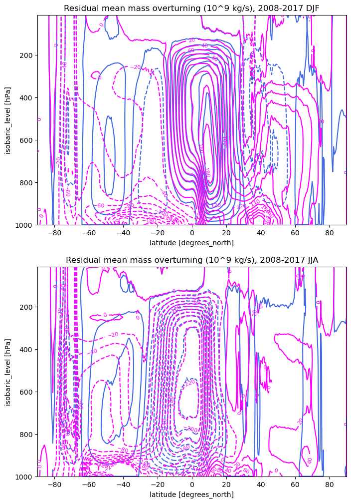
cluster.close()- Eliassen, A., & Palm, E. (1961). On the transfer of energy in stationary mountain waves. Geofysiske Publikasjoner, 22(3), 1–23.
- Edmon Jr., H. J., Hoskins, B. J., & McIntyre, M. E. (1980). Eliassen-Palm Cross Sections for the Troposphere. J. Atmos. Sci., 37, 2600–2616. https://doi.org/10.1175/1520-0469(1980)037<;2600:EPCSFT>2.0.CO;2