Earth’s radiation budget - ATM 622: General Circulation of the Atmosphere

Introduction¶

The “General Circulation of the Atmosphere” is the science of understanding the mean flow on scales from synoptic to global

What does it do?
What does it look like?
How do all the pieces fit together?

The circulation is fundamentally driven by two factors:

Differential heating via radiation
Rotation

In these notes we will begin exploring the first of those two factors: radiation and the energy budget of the Earth.

Earth’s Radiation Budget¶

Earth's Energy Balance — The global annual mean energy budget of Earth for the approximate period 2000–2010. All fluxes are in W m $^{–2}$ . Solar fluxes are in yellow and infrared fluxes in pink. The four flux quantities in purple-shaded boxes represent the principal components of the atmospheric energy balance. Source: Stephens *et al.* (2012)

Incoming solar radiation¶

Computing the incident sunlight hitting the Earth is a geometrical problem with a known solution so long as we know the details of the Earth’s orbit. For details, see this lecture in Brian Rose’s The Climate Laboratory

import numpy as np
import matplotlib.pyplot as plt
import xarray as xr

fsize = (10,6)  # A default figure size

import climlab

lat = np.linspace( -90., 90., 500)
days = np.arange(0., 1., 0.001) * climlab.utils.constants.days_per_year

Q = climlab.solar.insolation.daily_insolation( lat, days )

fig, ax = plt.subplots(figsize=(10,8))
CS = ax.contour( days, lat, Q , levels = np.arange(0., 600., 50.) )
ax.clabel(CS, CS.levels, inline=True, fmt='%1.0f', fontsize=10)
ax.set_xlabel('Days since January 1', fontsize=16 )
ax.set_ylabel('Latitude', fontsize=16 )
ax.set_title('Daily average insolation', fontsize=24 )
ax.contourf ( days, lat, Q, levels=[-1000., 0.], colors='k' );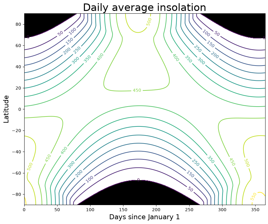

CERES EBAF data¶

The CERES-EBAF product is described by Kato et al. (2018).

# path_to_roselab = '/nfs/roselab_rit' # from DAES servers
path_to_roselab = '/Volumes/roselab_rit' # mounted on my laptop
ceres_URL = path_to_roselab + '/data/CERES_EBAF/CERES_EBAF_Ed4.1_200003-202202.nc'

ceres = xr.open_dataset(ceres_URL)
ceres

Computing monthly climatologies of CERES data¶

We can use Xarray’s groupby method to easily applying averaging operators over each calendar month.

solar_clim = ceres.solar_mon.mean(dim='lon').groupby("time.month").mean()
solar_clim

The monthly mean insolation as represented in CERES data¶

months = ['Jan', 'Feb', 'Mar', 'Apr', 'May', 'Jun', 'Jul', 'Aug', 'Sep', 'Oct', 'Nov', 'Dec']

fig, ax = plt.subplots(figsize=fsize)
levels = np.arange(0., 600., 50.)
CS = ax.contour(months, ceres.lat, solar_clim.transpose(), levels=levels)
ax.clabel(CS, CS.levels, inline=True, fontsize=10)

<a list of 32 text.Text objects>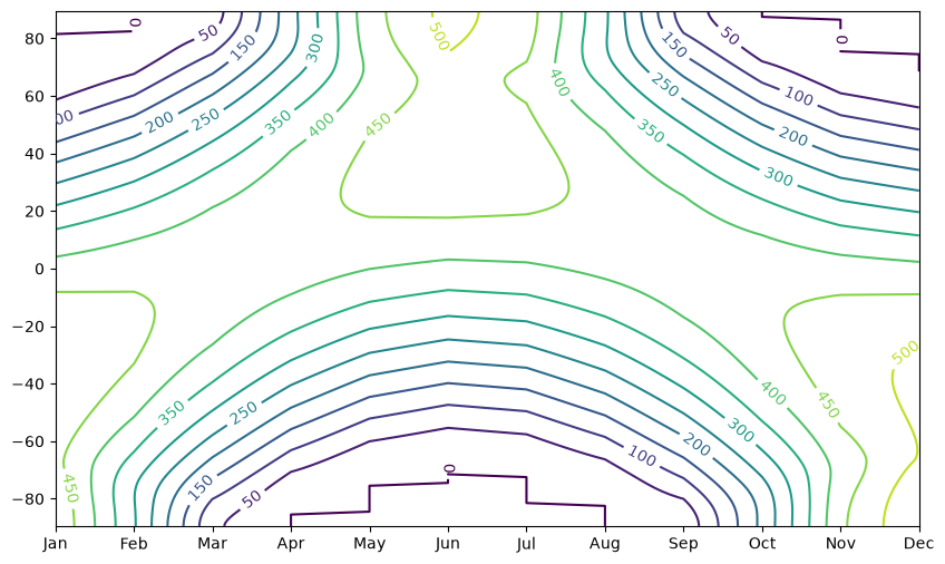

def annual_line_plot(da, title=''):
    '''A little helper function to make some nice line plots of annual means compared to January and July'''
    fig = plt.figure(figsize=fsize)
    da.mean(dim='month').plot(label='Annual', linewidth=3)
    for month_index in [0,6]:
        da.isel(month=month_index).plot(label=months[month_index])
    plt.legend()
    plt.xlim([-90,90])
    plt.grid()
    plt.title(title, fontsize=18);

annual_line_plot(solar_clim, title='Incoming solar radiation')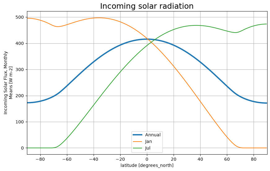

Albedo¶

The ratio of outgoing to incoming SW radiation:

\alpha = \frac{F_{SW}^{\uparrow}}{F_{SW}^{\downarrow}}

(1)

# masking out points where the insolation is near zero
ztoa_sw_all_clim = ceres.toa_sw_all_mon.mean(dim='lon').groupby("time.month").mean()

albedo = ztoa_sw_all_clim / solar_clim.where(solar_clim > 10.)  

annual_line_plot(albedo, title='TOA albedo')
plt.ylabel('Albedo');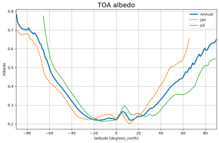

Absorbed shortwave radiation¶

The residual between what comes in and what goes out:

\text{ASR} = F_{SW}^{\downarrow} - F_{SW}^{\uparrow} = F_{SW}^{\downarrow} (1-\alpha)

(2)

absorbedSW = solar_clim - ztoa_sw_all_clim

annual_line_plot(absorbedSW, title='Absorbed shortwave flux')
plt.ylabel('flux (W m$^{-2}$)')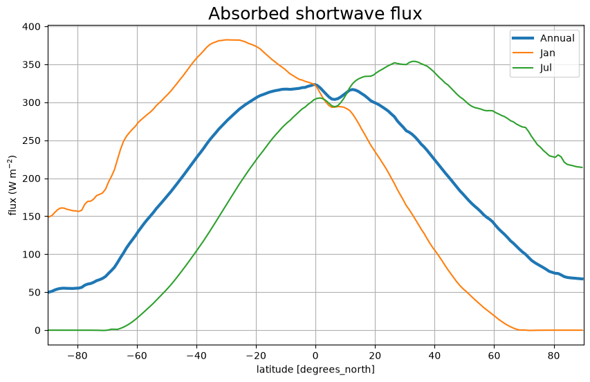

Outgoing longwave radiation¶

\text{OLR} = F_{LW}^{\uparrow}

(3)

ztoa_lw_all_clim = ceres.toa_lw_all_mon.mean(dim='lon').groupby("time.month").mean()

annual_line_plot(ztoa_lw_all_clim, title='Outgoing longwave radiation')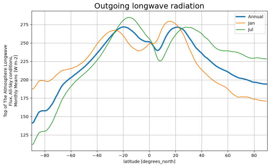

Net radiation at TOA¶

The net radiation is the difference between Absorbed Solar Radiation (ASR) and the Outgoing Longwave Radiation (OLR):

F_{net}^{\downarrow} = \text{ASR} - \text{OLR} = F_{SW}^{\downarrow} (1-\alpha) - F_{LW}^{\uparrow}

(4)

ztoa_net_all_clim = ceres.toa_net_all_mon.mean(dim="lon").groupby("time.month").mean()

annual_line_plot(ztoa_net_all_clim, title='TOA net radiative flux')
ylim = [-200, 200]
plt.plot([-90,90], [0,0], color='black')
plt.fill_between([-90,90], [ylim[0], ylim[0]], alpha=0.3, color='lightskyblue')
plt.text(-80, 160, 'net warming', fontsize=14)
plt.fill_between([-90,90], [ylim[1], ylim[1]], alpha=0.3, color='salmon')
plt.text(0, -140, 'net cooling', fontsize=14)
plt.ylim(ylim);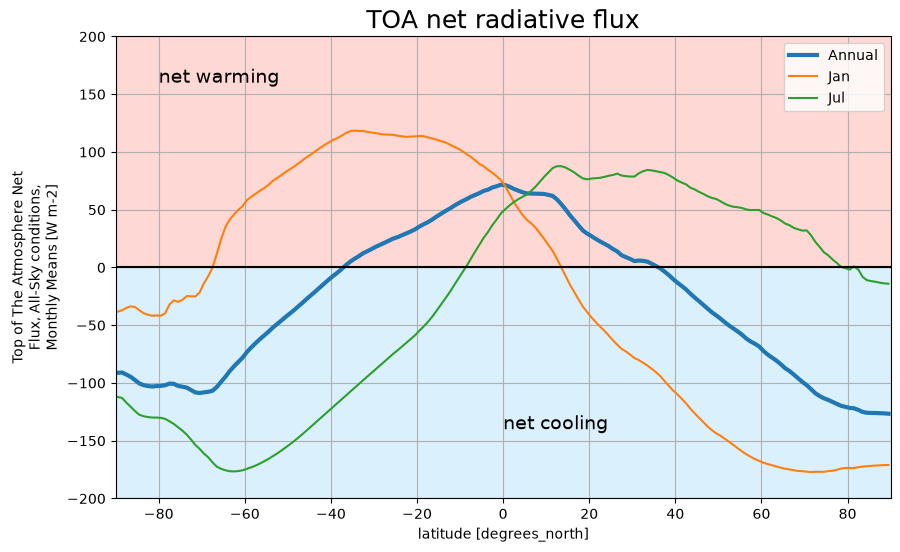

Hemispheric energy balance¶

Energy storage by latitude and season¶

A published version¶

Heat storage of the Earth–atmosphere system according to a 14 year average of CERES TOA net flux (in W m $^{−2}$ ) as a function of latitude and season. Source: Stephens & L'Ecuyer (2015)

And our own version based on the full CERES-EBAF dataset¶

fig, ax = plt.subplots(figsize=fsize)
CS = ax.contour(months, ceres.lat, ztoa_net_all_clim.transpose())
ax.clabel(CS, CS.levels, inline=True, fontsize=10)
ax.set_xlabel('Month', fontsize=16 )
ax.set_ylabel('Latitude', fontsize=16 )
ax.set_title('Heat storage of the climate system', fontsize=18 );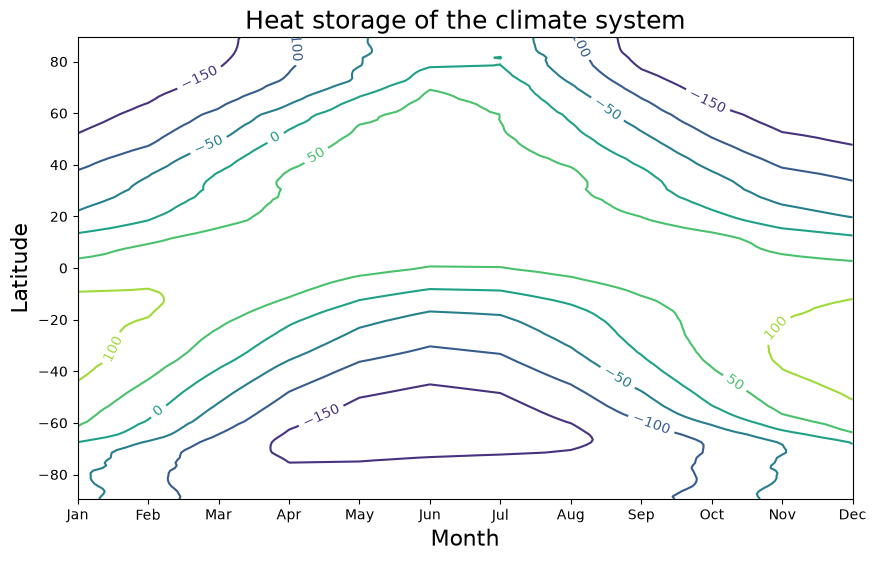

Meridional energy transport¶

Seasonal heat transport — The late February and August seasonal total heat transport: (a) shows the seasonal transports as highlighted and their average (thin solid line) contrasted against the heavy solid line representing the 14 year annual mean. The slight non-zero transport at the SH pole for both is indicative of the heat gained by the system. (b) The seasonal transports as in (b) highlighting the Tropical Trough Zone (TTZ) as a gray shaded region between 12 S and 20 N. Source: Stephens & L'Ecuyer (2015)

Precipitation and the ITCZ¶

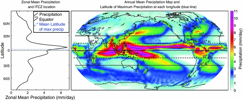
Annual mean precipitation — The annual mean precipitation from the National Oceanographic and Atmospheric Administration’s Climate Prediction Center’s (NOAACPC) merged analysis (Xie and Arkin 1996). Blue lines indicate the meridional location of the maximum in the Tropics at each longitude. The zonal mean is shown on the left and is co-plotted with the zonal mean of the local maximum (blue lines) and the precipitation centroid (dashed black lines). Source: Marshall *et al.* (2014)

Inferring energy transport from net radiation¶

The goal here is to demonstrate how we can infer a key property of the atmospheric and oceanic circulation using on the top-of-atmosphere radiative fluxes.

A volumetric energy budget and external sources¶

Consider a volumetric energy budget for the climate system in the form

\frac{\partial E}{\partial t} = S - \nabla \cdot (\vec{v} E)

(5)

where

$E$ is the energy per unit volume in the fluid (J m $^{-3}$ )
$S$ is the volumetric external energy source (W m $^{-3}$ )
$\vec{v} E$ is the total flux of the energy by the fluid (W m $^{-2}$ )
$\nabla \cdot$ represents the three-dimensional divergence

Averaging over a long period of time and assuming global energy balance, the left hand side is negligible so that

\nabla \cdot (\overline{\vec{v} E}) = \overline{S}

(6)

We are interested in the total transport including contributions from the bottom of the ocean to the top of the atmosphere. So, we integrate:

\int_{z_b}^{z_t} \nabla \cdot (\overline{\vec{v} E}) dz = \int_{z_b}^{z_t} \overline{S} dz

(7)

Since the only external sources to the entire column are at the top boundary, this gives

\nabla \cdot \int_{z_b}^{z_t} (\overline{\vec{v} E}) dz = \overline{F_{net}^{\downarrow}}

(8)

with $F_{net}^{\downarrow}$ the net downward flux of energy at TOA (W m $^{-2}$ ), and the divergence now two-dimensional in the latitude-longtitude plane.

Flux divergence in spherical coordinates¶

The flux divergence can be expressed in spherical coordinates as

\nabla \cdot \int_{z_b}^{z_t} (\vec{v} E) dz = \frac{1}{a \cos\phi} \frac{\partial}{\partial \lambda}\int_{z_b}^{z_t} u E dz + \frac{1}{a \cos\phi} \frac{\partial}{\partial \phi} \int_{z_b}^{z_t} v E \cos\phi dz

(9)

with this standard notation:

$a$ is the radius of the Earth
$\phi$ is latitude
$\lambda$ is longitude
$u$ and $v$ are the eastward and northward components of the velocity field

The total northward energy transport¶

We are interested in the total northward meridional energy transport, which is the integral of the meridonal component of the energy flux from the bottom of the ocean to the top of the atmosphere, and also integrating around the latitude circle:

\mathcal{H} = \int_0^{2\pi} \int_{z_b}^{z_t} a \cos \phi vE dz d\lambda

(10)

with the transport $\mathcal{H}$ now expressed in units of W.

So to see how $\mathcal{H}$ is related to the top-of-atmosphere radiative fluxes, multiple the energy balance equation through by the longitudinal arc length $a \cos \phi d\lambda$ and integrate around the latitude circle:

\int_0^{2\pi} \overline{F_{net}^{\downarrow}} a \cos\phi d\lambda = \int_0^{2\pi} \frac{\partial}{\partial \lambda}\int_{z_b}^{z_t} \overline{u E} dz d\lambda + \int_0^{2\pi} \frac{\partial}{\partial \phi} \int_{z_b}^{z_t} \overline{v E} \cos\phi dz d\lambda

(11)

and the first term on the RHS drops out (why?).

The zonal average¶

Let’s introduce some helpful notation we will use a lot.

Define the zonal average as the average of any quantity around the latitude circle:

[A] \equiv \frac{1}{2\pi} \int_0^{2\pi} A d\lambda

(12)

so we can write our integrated budget as

2\pi a \cos\phi [\overline{F_{net}^{\downarrow}}] = \frac{\partial}{\partial \phi} \int_0^{2\pi} \int_{z_b}^{z_t} \overline{v E} \cos\phi dz d\lambda

(13)

2\pi a^2 \cos\phi [\overline{F_{net}^{\downarrow}}] = \frac{\partial \overline{\mathcal{H}}}{\partial \phi}

(14)

Integrating the energy budget from the pole¶

We can now obtain the total northward transport $\mathcal{H}$ at any latitude by integrating our budget equation starting from the South Pole and working northward:

\overline{\mathcal{H}}(\phi) - \overline{\mathcal{H}}(-\pi/2) = \int_{-\frac{\pi}{2}}^\phi 2\pi a^2 \cos\phi [\overline{F_{net}^{\downarrow}}] d\phi

(15)

and, applying the boundary condition that the flux exactly at the pole must be zero, we get the result

\overline{\mathcal{H}}(\phi) = \int_{-\frac{\pi}{2}}^\phi 2\pi a^2 \cos\phi [\overline{F_{net}^{\downarrow}}] d\phi

(16)

which simply states that the northward energy transport at any latitude is balanced by the area-weighted top-of-atmosphere radiative imbalance accumulated from the pole.

References¶

Stephens, G. L., Li, J., Wild, M., Clayson, C. A., Loeb, N. G., Kato, S., L’Ecuyer, T., Jr., P. W. S., Lebsock, M., & Andrews, T. (2012). An update on Earth’s energy balance in light of the latest global observations. Nature Geoscience, 5, 691–696. 10.1038/NGEO1580
Kato, S., Rose, F. G., Rutan, D. A., Thorsen, T. J., Loeb, N. G., Doelling, D. R., Huang, X., Smith, W. L., Su, W., & Ham, S.-H. (2018). Surface Irradiances of Edition 4.0 Clouds and the Earth’s Radiant Energy System (CERES) Energy Balanced and Filled (EBAF) Data Product. J. Climate, 31, 4501–4527. 10.1175/JCLI-D-17-0523.1
Stephens, G. L., & L’Ecuyer, T. (2015). The Earth’s energy balance. Atmospheric Research, 166, 195–203. 10.1016/j.atmosres.2015.06.024
Marshall, J., Donohoe, A., Ferreira, D., & McGee, D. (2014). The ocean’s role in setting the mean position of the Inter-Tropical Convergence Zone. Climate Dynamics, 42, 1967–1979. 10.1007/s00382-013-1767-z