1. Climate models, the global energy budget, and Fun with Python#
This notebook is part of The Climate Laboratory by Brian E. J. Rose, University at Albany.
1. What is a Climate Model?#
First, some thoughts on modeling from xkcd

Let’s be a little pedantic and decompose that question:
what is Climate?
what is a Model?
Climate is
statistics of weather, e.g. space and time averages of temperature and precip.
(statistics might also mean higher-order stats: variability etc)
A model is
not easy to define!
Wikipedia: http://en.wikipedia.org/wiki/Conceptual_model
In the most general sense, a model is anything used in any way to represent anything else. Some models are physical objects, for instance, a toy model which may be assembled, and may even be made to work like the object it represents. Whereas, a conceptual model is a model made of the composition of concepts, that thus exists only in the mind. Conceptual models are used to help us know, understand, or simulate the subject matter they represent.
George E. P. Box (statistician):
Essentially, all models are wrong, but some are useful.”
From the Climate Modelling Primer, 4th ed [McGuffie and Henderson-Sellers, 2014]
In the broadest sense, models are for learning about the world (in our case, the climate) and the learning takes place in the contruction and the manipulation of the model, as anyone who has watched a child build idealised houses or spaceships with Lego, or built with it themselves, will know. Climate models are, likewise, idealised representations of a complicated and complex reality through which our understanding of the climate has significantly expanded. All models involve some ignoring, distoring and approximating, but gradually they allow us to build understanding of the system being modelled. A child’s Lego construction typically contains the essential elements of the real objects, improves with attention to detail, helps them understand the real world, but is never confused with the real thing.
A minimal definition of a climate model#
A representation of the exchange of energy between the Earth system and space, and its effects on average surface temperature.
(what average?)
Note the focus on planetary energy budget. That’s the key to all climate modeling.
2. The observed global energy budget#
The figure below shows current best estimates of the global, annual mean energy fluxes through the climate system [Trenberth and Fasullo, 2012].
We will look at many of these processes in detail throughout the course.
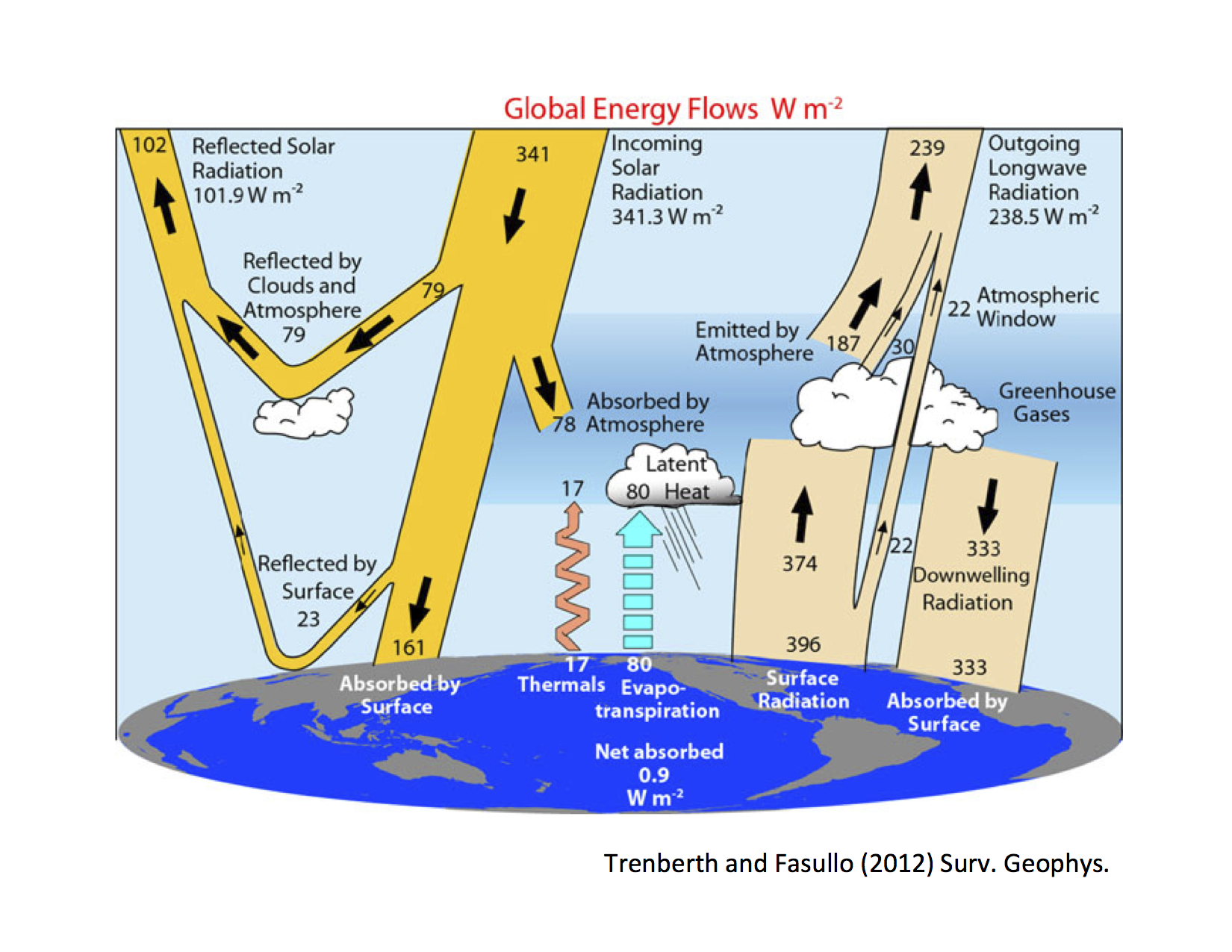
Things to note:#
On the shortwave side#
global mean albedo is 101.9 W m\(^{-2}\) / 341.3 W m\(^{-2}\) = 0.299
Reflection off clouds = 79 W m\(^{-2}\)
Off surface = 23 W m\(^{-2}\)
3 times as much reflection off clouds as off surface
Why?? Think about both areas of ice and snow, and the fact that sunlight has to travel through cloudy atmosphere to get to the ice and snow. Also there is some absorption of shortwave by the atmosphere.
Atmospheric absorption = 78 W m\(^{-2}\) (so about the same as reflected by clouds)
QUESTION: Which gases contribute to shortwave absorption?
O\(_3\) and H\(_2\)O mostly.
We will look at this later.
On the longwave side#
Observed emission from the SURFACE is 396 W m\(^{-2}\)
very close to the blackbody emission \(\sigma T^4\) at \(T = 288\) K (the global mean surface temperature).
BUT emission to space is much smaller = 239 W m\(^{-2}\)
QUESTION: What do we call this? (greenhouse effect)
Look at net numbers…#
Net absorbed = 0.9 W m\(^{-2}\)
Why?
Where is that heat going?
Note, the exchanges of energy between the surface and the atmosphere are complicated, involve a number of different processes. We will look at these more carefully later.
Additional points:#
Notice that this is a budget of energy, not temperature.
We will need to discuss the connection between the two
Clouds affect both longwave and shortwave sides of the budget.
WATER is involved in many of the terms:
evaporation
latent heating (equal and opposite in the global mean)
clouds
greenhouse effect
atmospheric SW absorption
surface reflectivity (ice and snow)
Discussion point#
How might we expect some of the terms in the global energy budget to vary under anthropogenic climate change?
3. Using Python to compute emission to space#
Most of what follows is intended as a “fill in the blanks” exercise. We will practice writing some Python code while discussing the physical process of longwave emission to space.
Suppose the Earth behaves like a blackbody radiator with effective global mean emission temperature \(T_e\).
Then
where OLR = “Outgoing Longwave Radiation”, and \(\sigma = 5.67 \times 10{-8}\) W m\(^{-2}\) K\(^{-4}\) the Stefan-Boltzmann constant
We can just take this as a definition of the emission temperature.
Looking back at the observations, the global, annual mean value for OLR is 238.5 W m\(^{-2}\).
Calculate the emission temperature \(T_e\)#
Rerranging the Stefan-Boltzmann law we get
First just use Python like a hand calculator to calculate \(T_e\) iteractively:
Try typing a few different ways, with and without whitespace.
Python fact 1#
extra spaces are ignored!
But typing numbers interactively is tedious and error prone. Let’s define a variable called sigma
Python fact 2#
We can define new variables interactively. Variables let us give names to things. Names make our code easy to understand.
Thoughts on emission temperature#
What value did we find for the emission temperature \(T_e\)? How does it compare to the actual global mean surface temperature?
Is the blackbody radiator a good model for the Earth’s emission to space?
A simple greenhouse model#
The emission to space is lower because of the greenhouse effect, which we will study in detail later.
For now, just introduce a basic concept:
Only a fraction of the surface emission makes it out to space.
We will model the OLR as
where \(\tau\) is a number we will call the transmissivity of the atmosphere.
Let’s fit this model to observations:
#tau = 238.5 / sigma / 288**4
Try calculating OLR for a warmer Earth at 292 K:
Naturally the emission to space is higher. By how much has it increased for this 4 degree warming?
Answer: 13.5 W m\(^{-2}\). Okay but this is tedious and prone to error. What we really want to do is define a reusable function
Note a few things:
The colon at the end of the first line indicates that there is more coming.
The interpreter automatically indents the code for us (after the colon)
The interpreter automatically colors certain key words
We need to hit return one more time at the end to finish our function
Python fact 3#
Indentations are not ignored! They serve to group together several lines of code.
we will see plenty of examples of this – in this case, the indentation lets the interpreter know that the code is all part of the function definition.
Python fact 4:#
def is a keyword that defines a function.
Just like a mathematical function, a Python function takes one or more input arguments, performs some operations on those inputs, and gives back some resulting value.
Python fact 5:#
return is a keyword that defines what value will be returned by the function.
Once a function is defined, we can call it interactively:
# print(OLR(288), OLR(292), OLR(292)-OLR(288))
Python fact 6#
The # symbol is used for comments in Python code.
The interpreter will ignore anything that follows # on a line of code.
Python fact 7:#
print is a function that causes the value of an expression (or a list of expressions) to be printed to the screen.
(Don’t always need it, because by default the interpreter prints the output of the last statement to the screen, as we have seen).
Note also that we defined variables named sigma and tau inside our OLR function.
What happens if you try to print(tau)?
Python fact 8:#
Variables defined in functions do not exist outside of that function.
Try declaring sigma = 2, then print(sigma). And try computing OLR(288) again. Did anything change?
Note that we didn’t really need to define those variables inside the function. We could have written the function in one line.
But sometimes using named variables makes our code much easier to read and understand!
Arrays with numpy#
Now let’s try some array calculations:
#import numpy as np
#T = np.linspace(230, 300, 10)
#print(T)
We have just created an array object.
The
linspacefunction creates an array of numbers evenly spaced between the start and end points.The third argument tells Python how many elements we want.
We will use the numpy package all the time. It is the basic workhorse of scientific computing with Python. We can’t do much with arrays of numbers.
Does our OLR function work on an array of temperature values?
Now let’s assign these values to a new variable.
#OLR = OLR(T)
Now try again to compute OLR(288)
What do you get?
Python fact 9: Assigning a value to a named variable overwrites whatever was already assigned to that name.#
Python is also case sensitive. If we had used olr to store the array, there would be no conflict.
Now let’s re-enter our function. Start typing def and then hit the “up arrow” key. What happens?
The editor gives us lots of useful keyboard shortcuts.
Here it’s looking up the last expression we entered that began with def. Saves a lot of time and typing!
Re-enter the function.
What happens if you use the up arrow without typing anything first?
Also, try typing history
This is very handy. The Python console is taking notes for you!
4. Summary#
Climate is essentially statistics of weather.
The planet warms up or cools down in response to differences between energy absorbed from the sun and energy emitted to space.
A climate model represents (mathematically of numerically) these exchanges of energy between the Earth system and space.
The observed emission to space or Outgoing Longwave Radiation is consistent with an emission temperature \(T_e = 255\) K – much colder than Earth’s surface.
This is evidence of the greenhouse effect.
We adopted a very simple greenhouse model, assuming a fixed transmissivity \(\tau\) for the atmosphere.
\(\tau\) conceptually represents the fraction of the emission from the surface that makes it all the way to space. It is a number less than 1.
Python is fun and useful.
Credits#
This notebook is part of The Climate Laboratory, an open-source textbook developed and maintained by Brian E. J. Rose, University at Albany.
It is licensed for free and open consumption under the Creative Commons Attribution 4.0 International (CC BY 4.0) license.
Development of these notes and the climlab software is partially supported by the National Science Foundation under award AGS-1455071 to Brian Rose. Any opinions, findings, conclusions or recommendations expressed here are mine and do not necessarily reflect the views of the National Science Foundation.